Introduction
The report aims at assessing the efficiency of an aluminium production plant utilising provided historical data for 2018 year. The dataset consists of a random sample of pots from four sections of the aluminium production plant from the previous year.
The present report contains a statistical analysis of provided data together with conclusions and recommendations concerning various aspects of aluminium production efficiency of the plant. We used the report brief provided by Colin Briggs to guide our assessment.
First, the report provides statistical data Grade-B and Chemical grade aluminium produced for each of the 4 sections separately and discusses its comparative performance. Second, we assess the current practice concerning cryolite purchase decision. Third, we evaluated if power consumption depends on the origin of cathode lining material. Finally, we identified if there is a linear correlation between bauxite consumption and total production. At the end of the report, we summarised our finding and provided recommendations based on data analyses.
We performed all calculations presented in the present paper using Microsoft Excel 2016 and Minitab 19. Even though Microsoft Excel 2016 has all the functions needed to analyse the data, we decided it was vital to double-check all the results using the latest statistical software, such as Minitab 19.
Grade-B and Chemical Grade Aluminium
Grade-B Aluminium
The first task mentioned in the report brief was to provide a summary statistical analysis of the Grade-B produced for each of the 4 sections separately and discuss these statistics. We analysed the performance of 80 pots with 20 pots in every section. The descriptive statistics for Grade B aluminium production is by section is represented in Table 1.1 below.
Table 1.1 – Grade-B Descriptive Statistics by Section.
The observations of the statistical data revealed that Section 1 produces maximum Grade-B aluminium (0.4197 tons), while pots from Section 4 produce considerably less Grade-B aluminium (0,3302 tons). In order to understand if there is a statistically significant difference between the means, we performed ANOVA analysis. Graphical representation of ANOVA analysis is presented in Figure 1.1 below.
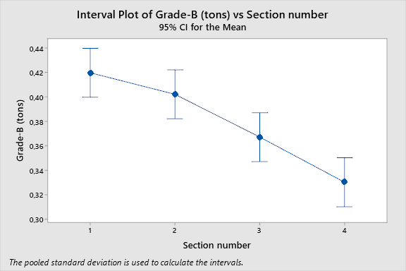
ANOVA analysis revealed that there is a statistically significant difference (p=0.000) between the means of Grade-B aluminium production in pairs of Section 1/Section 4 and Section 2/Section 4. The results suggest that the reasons for the low level of Grade-B aluminium production should be investigated and strategies for improving the performance identified.
Chemical Grade Aluminium
We analysed the production of chemical grade aluminium using similar methods as for Grade-B aluminium. Descriptive statistics of samples and ANOVA analysis are demonstrated in Table 1.2 and Figure 1.2 respectively.
Table 1.2 – Chemical Grade Descriptive Statistics by Section.
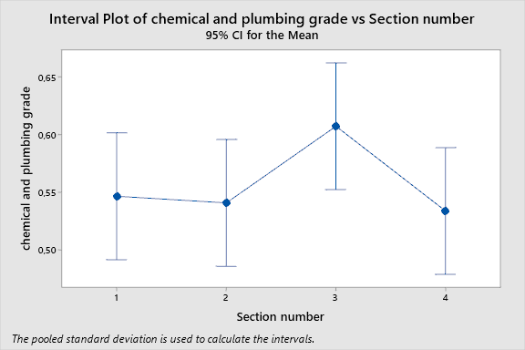
According to Table 1.2, the means of chemical grade production of aluminium are similar among sections, with a slight deviation in Section 3, where average output is 0.6073 tons per pot. At the same time, the section is characterised by having the highest range (0.4686 tons) of chemical grade aluminium production per pot. We found the matter concerning and decided to test if the difference in means was statistically significant. For this reason, we analysed the relevant data using ANOVA
The ANOVA analysis revealed no anomalies among the sections concerning the production of chemical grade aluminium. In other words, the differences in means of output are statistically insignificant. Therefore, we propose no interventions or regarding the production of this grade of aluminium.
Cryolite Consumption
The second part of the analysis aimed at determining how much cryolite per pot should be purchased to ensure uninterrupted operation of the plant and to optimise associated expenses. According to the report brief, current purchasing decisions are based upon an average cryolite consumption of 2.877 kgs per pot. In order to determine if the current policy is optimal, we calculated and juxtaposed the mean use of cryolite against the current supply level.
We performed one-sample t-test with two different levels of significance to assess the current practice. First, we tested the data using a confidence interval of 95% was (CI=95%). The results of the analysis are represented in Table 2.1 below.
Table 2.1 – Cryolite Use per Pot with CI=95%.
As observed in Table 2.1, when applying a 95% confidence interval, the average consumption of cryolite is between 2.4229 and 2.5449. We performed hypothesis testing with H₀: μ = 2.877 and H₁: μ ≠ 2.877. The results demonstrate that the current supply level of 2.877 is significantly higher (p=0.000) than the current level of consumption with a confidence level of 0.05.
Second, we tested the data using a confidence interval of 99% was (CI=99%). The results suggested that the mean cryolite consumption is between 2.4030 and 2.5648. The output of t-test hypothesis testing for CI=99% is demonstrated in Table 2.2 below.
Table 2.2 –One-Sample T-Test Results for CI=99%.
As can be seen in Table 2.2, the current supply level of 2.877 kgs is significantly higher than the current consumption level (p=0.000) with a significance level of 0.01. Therefore, we propose that the current practice is to be changed and the amount of cryolite purchased per pot decreased. Even though there is a possibility that provided historical data may be inconclusive, statistical analysis suggests that the practise should change to at most 2.565 kgs per pot. The number is the upper limit of CI=99%, which ensures continuous undisturbed plant operation. At the same time, 2.403 kgs of cryolite per pot (lower limit of CI=99%) is also a viable option if minimization if costs reduction is the top priority.
Cathode Lining Material
The third task mentioned by Colin Briggs was to determine if there is a statistical difference between the power consumption of pots that use locally produced material for cathode lining and those that use imported material. According to report brief, pots from section 1 and 4 utilise imported material, while pots from section 2 and 3 use locally produced substances. We compared the means of power consumption between the two groups of pots using a two-sample t-test.
In order to divide the pots into two groups, we added another variable to the dataset, which was called ‘Cathode Lining Origin.’ The additional variable helped to make automatic calculations in Minitab to ensure the most reliable results.
The calculations relied on the following assumptions: significance level of 0.05, equal variances, and sample size of 80.
The descriptive statistics for the two identified groups are represented in Table 3.1 below.
Table 3.1 – Descriptive Statistics of Power Consumption by Cathode Lining Origin.
We introduced two new variables to facilitate further tests:
- μ₁: mean of Power consumption (x 1000 kWh) when Cathode Lining Origin = Imported
- µ₂: mean of Power consumption (x 1000 kWh) when Cathode Lining Origin = Local
We identified the following hypotheses:
- Null hypothesis: H₀: μ₁ – µ₂ = 0
- Alternative hypothesis: H₁: μ₁ – µ₂ ≠ 0
The test results revealed that the p-value was 0.749, which is significantly higher than the significance level of 0.05. This implies that we cannot reject the null hypothesis. Therefore, data analysis concluded that there is no statistically significant difference in power consumption between the two different types of cryolite.
Relationship between Bauxite Consumption and Total Production
Identifying the Variables
The final task mentioned in the report brief was to determine if there is a linear relationship between aluminium production and bauxite consumption. In order to complete the task, we decided it was necessary to introduce a new variable, which we called ‘Total Production’. We calculated the variable by adding the output of all alloy and non-alloy grades of aluminium included in the dataset. After that, we identified that regression analysis was needed to identify if one of the values can predict the other using a linear model.
As it is commonly known, regression analysis requires having an explanatory variable and a response variable. In other words, one of the variables is to be independent, which implies that they remain unaffected by other variables. In contrast, response variables are dependent, in the sense that other variables may influence them. Following this logic, we identified bauxite consumption as the explanatory because other variables cannot influence the amount of material. We also treated total production as the response variable since it can supposedly be predicted by bauxite consumption.
Regression Equation
In order to identify if a linear correlation is possible between the two variables, we conducted a regression analysis and created an equation. The general linear regression equation looks as follows:
y = mx + b
Where y is the response variable, x is the explanatory variable, m is the slope of the regression line, and b is the value where the regression line intercepts with the y-axis. We conducted a regression analysis using Minitab 19 to calculate m and b. The output of the analysis is represented in Table 4.1 below.
Table 4.1 – Regression Analysis Output.
Using the data in Table 4.1, we created a regression line equation, which is the following:
Total Production = 1.253*Bauxite Consumption – 3.14
The equation indicates that when the gradient of the line is 1.253 and bauxite consumption is equal to 0, the regression line below intercepts the Y-axis at the point (0, -3.41). Hence, if the bauxite input increases by 1 then the total production will increase by 1.253.
Evaluation of the Regression Model
In order to evaluate the predictability of total production using bauxite consumption, we decided to create a scatterplot and the regression line on the same chart. The chart is represented in Figure 4.1 below.
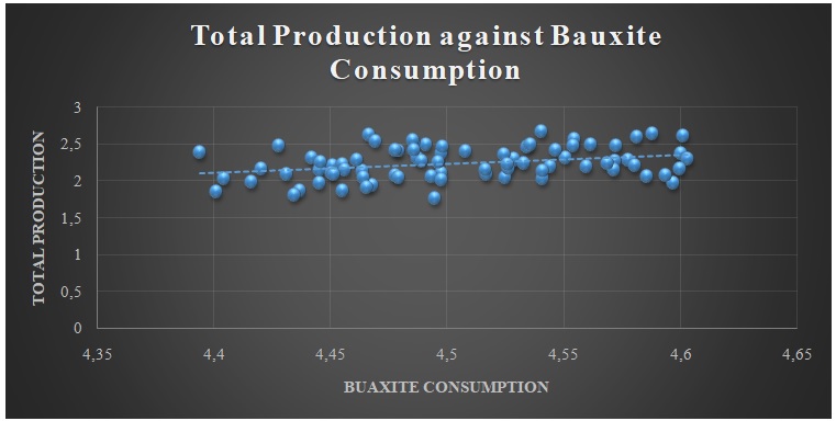
As one can see in Figure 4.1, the provided regression line is not an adequate fit for the data. Even though there some dots that are close to the regression line, the majority of data is dispersed. This implies that the correlation between the two variables is weak.
In order to confirm the assumption, we assessed the regression statistics. In particular, we paid careful attention to R2 and adjusted R2 coefficients. R Square and adjusted R2 the statistic that evaluates the amount of correlation (ranging from 0 to 1). The results of the analysis are shown in Table 4.2 below.
Table 4.2 – Regression Line Model Summary.
According to Table 4.2, R2 is equal to 0.1052, which is significantly less than 1. In other words, only 10.52% of changes in total production can be explained by variations in bauxite consumption. Therefore, statistical analysis confirms that the correlation between variables is weak.
While the relationship between the two variables is weak, there is no basis to declare that the correlation is absent. In order to prove that the relationship is statistically significant, we performed two hypothesis tests:
- Null hypothesis: H0: β1=0;
- Alternative Hypothesis: H1: β1≠0, where β1 is the P-value;
The calculation revealed that the P-value is 0.003, which is smaller than the significance level of α= 0.05. Therefore, we should reject the null hypothesis and accept the alternative hypothesis. In conclusion, the statistical analyses demonstrate that even though the relationship between the variables is weak, it is statistically significant.
Regression Model Assumptions
The primary assumptions that should be taken into account are as follows:
- The variance remains constant;
- The residuals are independent of bauxite consumption;
- The residuals are normally distributed;
In order to assess the variance and dependence of residuals from bauxite consumption, the residual plot was created using Microsoft Excel. If the variance is equal, the points should be dispersed evenly along with the rage of X (bauxite consumption). Moreover, a clear pattern should not be seen that can confirm the dependence of residuals from bauxite consumption. The plot is shown in Figure 4.2 below.
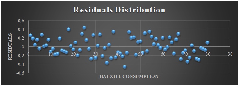
The observation of Figure 4.2 shows that there is no clear pattern that can be seen on the chart. Therefore, we concluded that residuals are independent of bauxite consumption. However, the points are not equally dispersed along the X line, which implies that the variances are not equal.
Furthermore, we assessed the distribution of residuals to identify if it followed a normal distribution curve. In order to achieve that, we created a histogram of residual distribution along the X-axis. The chart is represented in Figure 4.3 below.
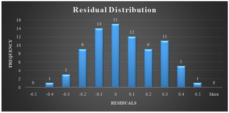
As observed in Figure 4.3, residual distribution resembles the normal distribution curve. Therefore, we concluded that the third assumption was correct and the residuals are normally distributed.
Summarising the analysis of residuals, we concluded that the validity of regression analysis is questionable. The reason for the conclusion is that 1 out of 3 assumptions was not met, which implies that the data analysis is biased at a certain extent.
Predictions
While the validity of the regression model is low, it can still be used to make predictions for total production using the data concerning bauxite consumption. First, the report brief asks for total production using the bauxite consumption for pot 414 in Section 4, which is 4.401057. After applying the regression model, we received the following results:
Total Production = 1.253*4.401057 – 3.41 = 2.1045 tons
When juxtaposed with the actual total production of 1.8557, we observed a significant difference between the two values demonstrate the low validity of the calculated regression model.
Furthermore, Colin Briggs mentioned that predictions for bauxite input of 4.2 and 4.8 were needed. The calculations for the predictions are demonstrated below:
For bauxite consumption of 4.2 tons,
Total Production = 1.253*4.2 – 3.41 = 1.8526 tons
For bauxite consumption of 4.8 tons,
Total Production = 1.253*4.8 – 3.41 = 2.6044 tons
While the predictions may have a certain degree of accuracy, they should be used with caution due to low predictability of the regression model.
Conclusions and Recommendations
Before introducing findings and recommendations, we want to restate that the present report was based upon aggregated data of the performance of the aluminium plant during one year. In order to acquire more precise results, we recommend using data from several years of plant’s operations. However, we identified the provided sample size as sufficient to make conclusions with adequate generalizability level.
First, the observations of descriptive statistics concerning the production of chemical grade aluminium and Grade-B aluminium revealed underperformance of pots from Section C and D in terms of Grade-B aluminium production. We recommend investigating the reasons for the matter using methods provided by statistics and beyond to improve the current output if needed.
Second, we assessed the current policy concerning cryolite purchases per pot. We identified that the plant should decrease the purchases of cryolite to the level between 2.4030 and 2.5648, depending on the company’s priorities.
Third, we identified that the origin of cathode lining material (local against imported) does not influence power consumption. Therefore, we recommend basing the decisions concerning cathode lining material on other matters, such as price and availability.
Finally, we created a regression model to predict total production using bauxite input levels. The analysis revealed that the correlation between the two matters is weak. Therefore, we recommend that the provided model should not be used for prediction purposes.