Abstract
This paper discusses a company that purchases houses, repairs them, and resells them at a higher price afterward to make profits. It is in need of a model that can predict several essential characteristics of a house, most importantly the repair cost and the profit that can be made from it. To that end, the H2O package was used to create a model that takes a number of inputs and produces a prediction of these characteristics. The number of bedrooms, age of the house, purchase price, and its size were expected to be the most significant factors for the profit. The size was also considered an essential predictor of the repair cost, which was confirmed in the preliminary investigation. A Gradient Boosted Machine algorithm was used to arrange the potential predictors in order of significance. The model was able to isolate multiple vital factors that affect the profits, such as the house size, repair costs, and the number of bedrooms, garages, and bathrooms. However, there were no significant predictors for the repair costs, most likely as a result of the low sample size and the lack of detailed variables. It is likely impossible to use the model for repair costs used the nature of the business, but, barring investigation into some notable outliers, it appears to be appropriate for comparing potential profits if the repair cost is estimated manually.
Introduction
Buy N Sell is a business that operates by purchasing houses in disrepair at a low price, fixing them, and reselling them at a higher price to make a profit. It relies on investors to provide the sums for the house purchases and finance the repairs, as this structure enables it to operate with improved flexibility. As such, to retain their interest, the business has to consistently produce high profits that remain attractive compared to other options. As such, the firm considers any project that generates less than $20,000 in profit to be a failure. However, as Trim (2018) notes, the so-called “house flipping” is a risky affair, as it relies on correctly identifying attractive homes, purchasing them below market price, and avoiding overcapitalization. The company is interested in determining the factors that can help it predict whether it can reach its target profit figure based on specific house characteristics.
The project’s primary objective is to identify the relationship between various aspects of a house and its ability to generate a profit for the business. Its first research question is what factors best predict the overall cost of repairs that will need to be done to make the house suitable for resale. Second, it will investigate what characteristics of a home best determine its purchase and sale prices. Using this information, the company will be able to quickly and efficiently choose the most suitable locations for its operations and conduct high-profit operations.
Methodology
The study will be quantitative in nature, aiming to estimate the relationship between various house traits and qualities and the profit that can be made from the property. In order to gather information about houses, the data for the project were collected using the records of the last three years of Buy N Sell’s operations. They feature general information about 62 houses, such as their purchase and sale prices, repair expenses, and measurements such as size and number of bedrooms. With that said, 12 of those houses had to be eliminated due to various reasons, such as inadequate information, leaving a sample of 50. Additionally, the company’s experts have been collecting detailed information about houses that they worked on, such as the number of light fixtures, flooring and landscaping quality, and others. In the future, they will continue doing so and feeding the data into the model to improve its accuracy.
First, it is necessary to determine whether the different variables should be classified as continuous or categorical. The characteristics that are expressed with small integer numbers, namely the numbers of bedrooms, bathrooms, and garages, should be categorical by their nature. Factors that are based on a subjective evaluation, notably the quality of the flooring, should also be categorical, as that is how most people would arrange them already. On the other hand, the approximate cost of the appliances, the number of light fixtures that need to be replaced, and the owners’ offered sale price should be continuous. The size of the house should be continuous, as prices are often determined on a per-square-foot basis. Its age was separated into two distinct categories, based on whether it was constructed before (0) or after (1) 1995, using data discretization (Miner et al., 2017) to broadly evaluate its attractiveness and degree of repairs likely needed. Lastly, the target variables, namely the recommended purchase and resale prices as well as the repair costs, should be continuous.
The problem that is being considered in this report is one of estimating a set of numbers given particular inputs. However, these starting values are immutable, and the program is being asked to guess the results using the relationships it finds between the different variables instead of trying to optimize them. Per Boehmke and Greenwell (2020), this requirement places the problem in the dimension reduction category of unsupervised learning. It aims to separate the most significant correlations between the different variables and eliminate those that exert little to no influence. By selecting specific items and examining their set of relationships, the user can then determine the factors that influence their desired outcomes the most and consider them in future endeavors.
To create the model, the H2O package will be used to develop and train a number of different models that are based on the various algorithms available. They will first progress independently, using the same portion of the data set to produce potentially meaningfully different results. Next, cross-validation will be used with the remaining parts of the sample to ensure that the models are valid and produce somewhat accurate results. Following this procedure, two stacked ensembles will be created: one that contains all the models and one that has the best one from each algorithm class. After training these ensembles, H2O will produce a leaderboard of the models that have generated the best results and a list of variables ranked by their ability to predict profit. The project’s authors are particularly interested in the relationship between profit and the number of bedrooms as well as the age, cost, and size of the house.
A Gradient Boosted Machine algorithm was used to order the possible predictor variables from the most important variable to the least important for the response variable “Profit”. With the factors that determine profit identified, the project can proceed to evaluate their relationship with profit in more specific terms. To test these hypotheses, a generalized linear model was used with an inverse gaussian family and a log link function, due to the right skewness of the response variable (profit). A generalized linear model is used to find the particular degree to which changes in predictive variables correspond to differences in the profit made.
The most significant problem that the project is expected to encounter is the relatively low sample size. It takes a substantial time to repair a house, particularly considering Buy N Sell’s somewhat small workforce. As such, the company cannot provide a large database of houses on which it has worked that would normally be considered adequate for a machine learning project. In the future, the model will be updated as the company uses it to select houses and work on them, but the rate of the sample’s growth will still be slow. As such, there are highly likely to be substantial biases that hinder the model’s accuracy. Still, it should be able to produce a model that is adequately accurate for the business’s needs and can be refined in the future.
Simulation Study
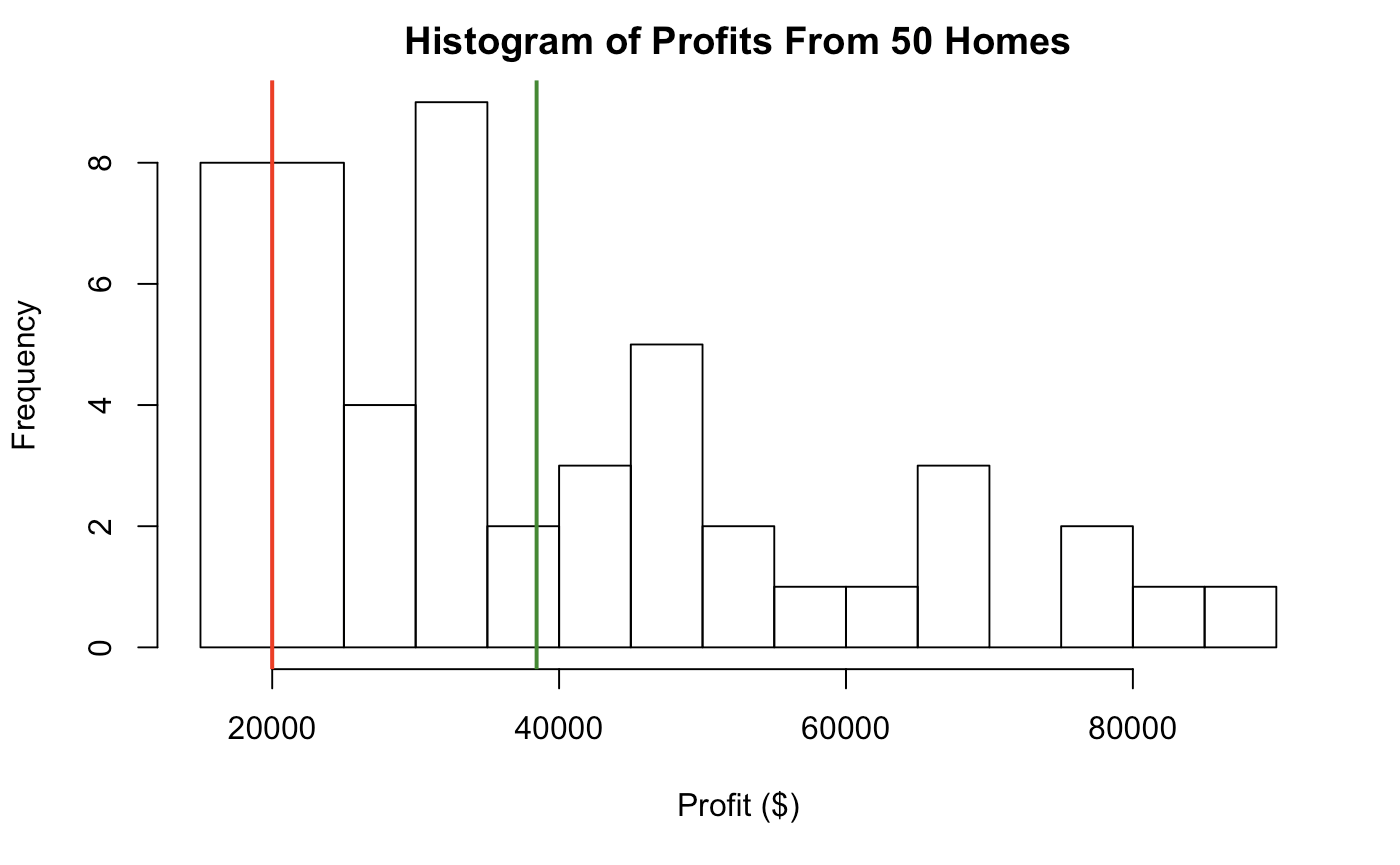
First, a study of the houses that constituted the database took place to isolate some findings and obtain a better understanding of the model’s conclusion. First, the houses were sorted based on the profits that they have generated, the result of which is shown in Fig. 1. The average profit for 50 homes from the selection was $38432.23, represented by the green line, and the standard deviation was equivalent to $18852.64. Profits below $20,000 were determined to be unacceptable and are represented by the red line in the histogram. They range between a maximum of $88580.03 and a minimum of $17523.42.
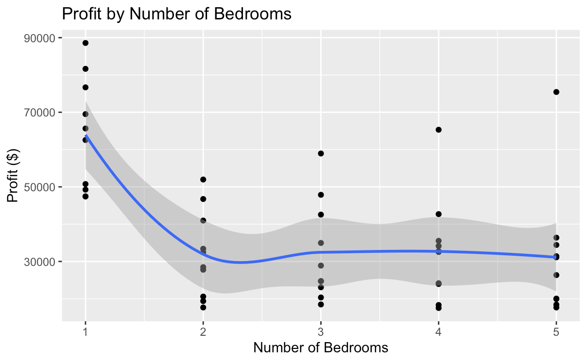
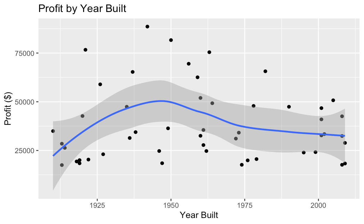
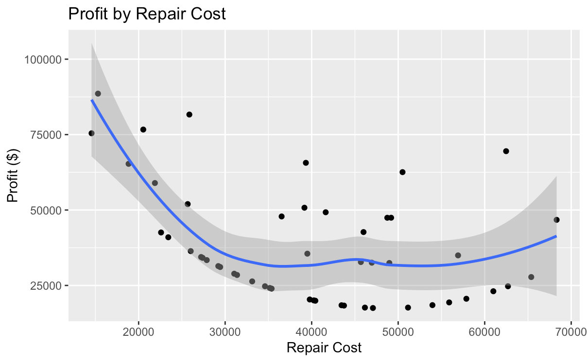
Next, the author selected several characteristics that they considered likely to be highly influential and investigated their relationship with profit. They found that, as shown in Fig. 2, among all houses, houses with one bedroom generated substantially higher profits than those with other counts, both individually and on average. Additionally, houses that were built in the late 1940s produced higher profits than the rest, as Fig. 3 demonstrates. This finding is anomalous and will be viewed as an outlier, as it would potentially skew the model toward older houses if it were considered. Lastly, Fig. 4 demonstrates the relationship between repair costs and profit, showing that houses that are cheaper to fix generate substantially higher income for the company.
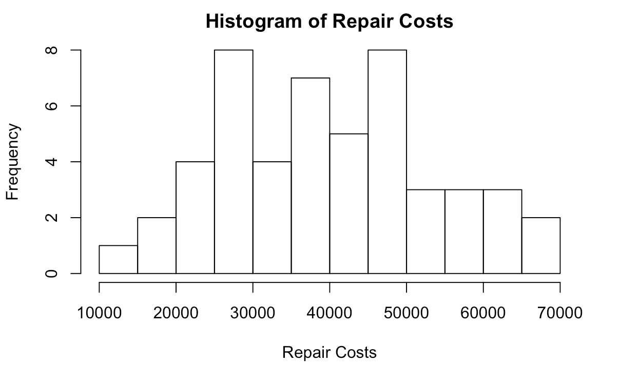
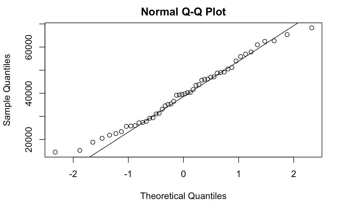
The author also investigated the relationship between the size of the house and the costs of repairing it. They found that the repair costs appeared to follow a normal distribution of costs, with a majority between $25,000 and $50,000, as shown in Fig. 5. When constructing a scatter plot of house repair costs based on its size, the author generated the graph depicted in Fig. 6. It appears that there is a linear increase in the costs of a house’s repairs as its size grows. As such, a linear model, also depicted in Fig. 6, appears to be appropriate, suggesting a corresponding relationship between the two variables.
Next, the author ran the model and let it determine the factors that it considered most significant for determining that a house can generate. The results that it produced were repair costs, number of bedrooms (1), number of garages (1), number of garages (0), number of bathrooms (1), purchase price, lot size, house size, house age (1), and number of bedrooms (5). As demonstrated in the preliminary section, houses with one bedroom were determined to generate high profits, as were those that had low repair costs. However, with the outlier eliminated, the model found newer houses to generate higher profits than older ones. The size of the house (in square feet) was the most significant predictor of profits, with its p-value was below 0.05. Other factors that also satisfied this significance criterion were the repair costs as well as the number of garages and bathrooms. Moreover, the model as a whole was able to produce a p-value of 0.008, which is strongly statistically significant.
Following this step, the author chose to isolate the six most significant variables and limit the model to using them for predicting profits. These six items were the house size, lot size, purchase price, and the number of garages, bathrooms, and bedrooms. To test the appropriateness of the simplified model, the author calculated the Akaike information criterion. When all of the predictors were included, it was equivalent to 1042.296, and with the six most important ones, it fell to 1037.908, marking the six-predictor approach as superior to the more comprehensive alternative. As such, it was chosen for the purposes of the project and used in the final model.
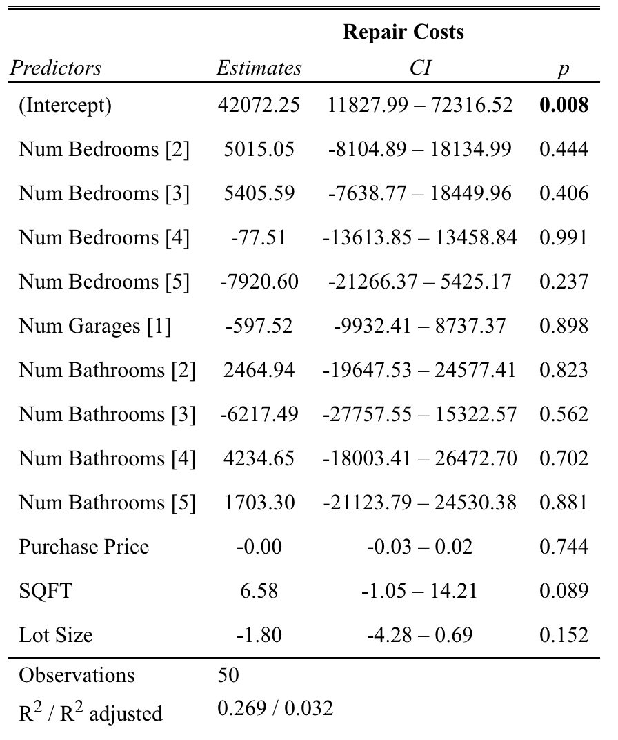
The model was also used to formulate a relationship between the most significant predictors and the repair costs of a house. As is shown in Table 1, none of the factors considered were significant for predicting the value. The size of the house in square feet (represented by SQFT) was the closest, with a p-value of 0.089, but it was still substantially above the required threshold of 0.05. Moreover, the R-squared coefficient for the model is 0.269, which is substantially lower than what is generally considered acceptable. As such, the model cannot be considered valid for the prediction of repair costs, either in its full form or in the simplified variety.
Conclusion & Limitations
First, it is necessary to discuss the results that the author was able to generate in the manual analysis. The reason why one-bedroom houses generate considerably more profits than their larger counterparts may be due to higher demand. Single people and families without young children are likely to be interested in purchasing such a house, possibly exceeding supply and being willing to pay more to secure it. With that said, this notion does not explain why the purchase price of such a house does not rise along with its resale price. A number of answers are possible for the relationship between house age and profit, but without evidence, none of them may be considered decisive. Lastly, the high profits associated with low repair costs may indicate that owners overestimate the repair costs of houses and are willing to sell them below their value.
The model was able to produce substantial results that do not necessarily confirm what was found in the preliminary analysis. The author expected the age of the house to be a significant predictor, but the model has not found it to be as important. It is possible that this result emerged because of the author’s elimination of the outlier houses that were constructed in the 1940s. As shown in Figure 2, profits made on newer houses tend to decline relative to prior times even if the anomalous period is eliminated. It is possible that the actions the author took introduced a form of bias in the model. Alternatively, there is a possibility that the model was able to identify a trend that the author was unable to recognize.
With regard to the repair costs, the author expected to find a significant relationship between the size of the house and the repair costs. The underlying idea was that larger houses have more points of failure and are, therefore, likely to manifest more breakages and elevate repair costs. The findings of their evaluation confirmed this notion, with the costs distributed normally and adhering to a linear distribution. However, the model rejected house size as a predictor of repair costs, contradicting the theoretical findings. It presumably found a weak correlation between the two values that were not strong enough to base the relationship on, with the others producing worse results. The author believes that the cause is the lack of information currently provided by the model. It omits factors that can contribute significantly to the repair costs, such as the condition of the piping or the electrical grid. When these factors are collected and entered into the system in the future, the model may clarify the relationship between house size and repair costs using these other variables.
Overall, the model is currently partially adequate for usage in a practical environment. It has found multiple significant predictors for the profit that can be made from a house and can be applied for that purpose. However, the model has failed in its secondary purpose of predicting the repair costs of a house. The R-squared value for this application is 0.269, which represents a low degree of predicting power for the independent variables chosen. It can be concluded that the problem of repair costs was not suitable for machine learning due to an inadequate sample and a lack of variables. This situation may change in the future, but, due to the nature of Buy N Sell’s business, it would take a change in operating strategies and a substantial amount of time to achieve this goal. As such, it can be concluded that it can be used for estimating profits and comparing houses based on them, but the repair costs need to be determined and entered manually.
References
Boehmke, B., & Greenwell, B. M. (2020). Hands-on machine learning with R. CRC Press.
Miner, G., Yale, K., & Nisbet, R. (2017). Handbook of statistical analysis and data mining applications (2nd ed.). Elsevier Science.
Trim, A. (2018). Real estate dangers and how to avoid them: A guide to making smarter decisions as a buyer, seller and landlord. Wiley.