To identify the best way to educate elementary-age children in mathematics, a researcher decides to conduct a pilot study among fifth-grade children throughout a school district. The researcher thinks that fifth-grade girls do better in small class sizes while boys perform well in larger classes. The pilot study involves classroom sizes that have been reduced into three groups. The first group is made of no more than 10 children; the second group has 11 to 19 children while the third group is made of 20 or more children. Using data collected from the pilot study, factorial ANOVA analysis on the data has been performed and presented in this paper. In addition, this paper presents a hypothetical ANCOVA based on variables that can help determine whether one will become delinquent.
Exploratory data analysis
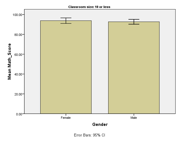
The mean math score for girls learning in classes of 10 or fewer children is 93.80, N = 10 whereas the standard deviation is 3.94 (Table 1). Table 1 also indicates that the minimum math score for girls in classes of 10 or fewer children is 88.00 while the maximum score is 98.00. The skewness is -.250 while the kurtosis is -1.688 (Table 1).
For male children studying in classes of 10 or fewer children, the mean math score is 92.70, N = 10 while the standard deviation is 3.43 and a variance of 11.79. The minimum math score is 87.00 and the maximum score for the same class is 99.00. From the same table, it is evident that the skewness is.195 whereas the kurtosis is.331. Figure 1shows a visual display of the mean math scores for children learning in a class of 10 or fewer children and it is evident that the mean math score for girls is only slightly higher than that of boys.
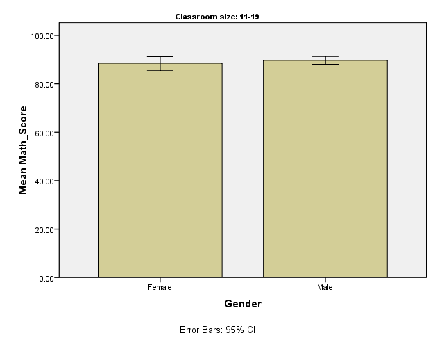
From Table 3, the mean math score for girls learning in classes of 11-19 children is 88.50, N = 10 and a standard deviation of 3.98 with a variance of 15.83. The minimum math score for this group is 82.00 and the maximum score is 95.00. The table also indicates the skewness for this data as -.026 and a negative kurtosis value of.670.
The mean math score for boys learning in classes of 11-19 children is 89.70, N = 10 and the standard deviation is 2.41 with a variance of 5.79. The maximum math score for this group of children is 93.00 and the minimum score is 86.00. The kurtosis is -1.269 and the skewness value of -.278. For children studying in classes of 11-19 children, it is clear from Figure 2 that the mean math score for boys is slightly higher than that of girls.
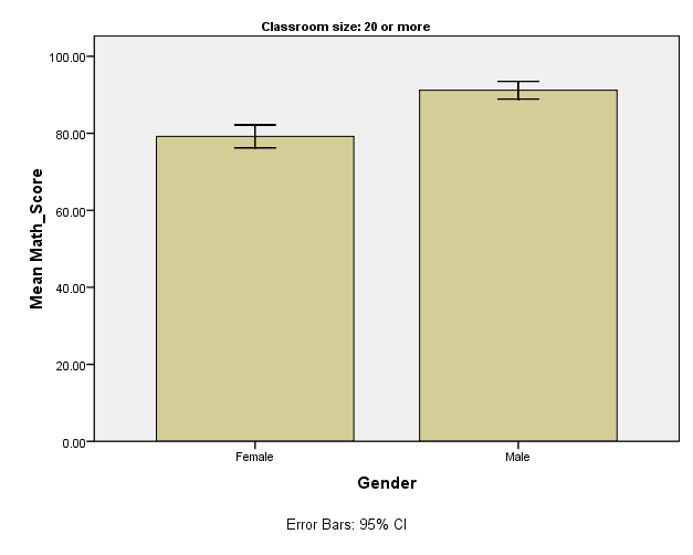
When learning in classes of 20 or more girls, the mean math score is 79.20, N = 10 and a standard deviation of 4.184 with a variance of 17.511. The maximum score attained by girls in classes of 20 or more children is 86.00 while the minimum score is 72.00. The skewness and kurtosis are negative values of.335 and.207 respectively.
Table 6 indicates that the mean math score for boys in classes of 20 or more children is 91.20, N = 10 and the standard deviation is 3.22 while the variance is 10.40. The minimum math score in this group is 87.00 and the maximum score is 98.00. The skewness and kurtosis are positive values of.918 and 1.016 respectively. A visual display of math scores for children in classes of 20 or more children in Figure 3 shows that the mean math score for males is distinctively higher than that of girls.
In summary, the math performance of girls declines as the class size increases whereas it is clear that the math performance of boys in small classes is almost the same as in large classes.
Factorial ANOVA
From the output in Table 9, it is evident that there is a main effect of gender. In other words, the main effect of gender was significant, F(1, 54) = 19.06, p<.05, indicating that when classroom size is ignored, math performance differs depending on whether the class is made of girls or boys. In this case, there is no need to use post-hoc tests to explain the effect since post hoc tests are not performed for variables that have fewer than three groups (Field, 2009). Table 8 shows that Levene’s test is not significant p =.539 and this is greater than .05 implying that homogeneity of variance can be assumed.
According to Tukey HSD test in Table 10, there is a significant difference in math performance when comparing a class size of 10 or fewer children with a class of 11-19 children (p =. 002). Similarly, Table 10 shows that there is a significant difference in math performance considering a class of 10 or less against a class of 20 or more students (p =. 000). Tukey test also shows that a significant difference (p =. 003) exists when comparing math performance between a class size of 11-19 children and that of 20 or more children. Games-Howell’s test also indicates that there is a significant difference (p =. 001) in exam performance when the class size is 10 or fewer children against a class size of 11-19 children.
Games-Howell test (Table 10) shows that there is no significant difference in exam performance when comparing a class size of 11-19 children against that of 20 or more children (p =. 086 which is greater than.05). Dunnett’s test however shows a significant difference in math performance (.002) comparing a class size of 11-19 children against 20 or more when the class of 10 or less is the control. When the class size of 11-19 children is the control, the difference between math performance in a class of 10 or less against a class of 20 or more children is significant (p =. 000).
There exists a main effect of classroom size as indicated in Table 9. To be precise, the main effect of classroom size is significant, F(2, 54) = 25.31, p<.05, indicating that math performance (ignoring the gender of the child) changes depending on whether the child is in a class of 10 or less, 11-19 or 20 or more children. Since classrooms have been grouped into three groups, post-hoc tests are necessary to explain the effect of classroom size.
There is an interaction between gender*classroom size and this interaction is significant, F(2, 54) = 19.10, p<.05. This indicates that the gender of the child combines with classroom size to affect math performance. Post-hoc tests indicate that for female children, math performance becomes poorer as the size of the class increases. The performance is best in classes of 10 or fewer children and worst in classes of 20 or more children.
For boys, the performance is best when the class size is both classes of 10 or fewer children and 20 or more children. It is for this reason that the researcher’s hypothesis (girls would do better than boys in classrooms with fewer students) has been rejected. Instead, the performance of girls in small classrooms is almost equal to that of boys in small classrooms. However, boys would indeed perform better in larger classes compared to girls’ performance in larger classrooms.
Research in My Area of Interest
I have an interest in working as an International Police Advisor (IPA) for the benefit of our Homeland Security. As an International Police Advisor, there are several responsibilities that I will be required to handle. Partnering with the U.S. military personnel to provide skilled persons in civilian law enforcement will be one of the main responsibilities. International Police Advisors can serve in Border and Point of Entry to enhance law at the borders and particularly prevent the entry of illegal persons, drugs, and weapons among other crimes. A great concern to the United States Homeland Security has been the identification of persons who are likely to engage in acts of terrorism or general crime.
Positive identification of likely criminals requires a thorough understanding of human behavior. In specific, an understanding of past criminal activities can be used to predict the likelihood of engaging in unlawful practices. In relation to my area of interest as an IPA, I would suggest conducting research to identify whether there is any relationship between prior engagement in misconduct, past experiences and delinquency and the likelihood of engaging in serious criminal activities.
This can form a concrete and dependable ground for criminal investigations. In this study, it would be advisable to examine an individual’s prior marriage relationships in order to predict involvement in crime. This is based on Sampson and Laub (1993) argument that if persons who are in the verge of entering adulthood get involved in marriage relationships, their likelihood in engaging in crime is significantly reduced. As such, persons with unstable or no marriage relationships in the transitory period are more likely to engage in criminal activities.
Xu (2006) observes that there is tendency of having persistent antisocial behaviors in the entire life of a person. In that case, it is possible to study the existence of juvenile delinquency as a predictor of adulthood delinquency. On the same aspect, identifying various social factors such as social networks as well as social capital would help predict involvement in criminal behaviors. In addition, this study would look into whether gender influences involvement in antisocial activities. From the understanding of the above questions, it would be possible to prevent criminals from perpetrating their heinous acts thus proving beneficial to the Department of Homeland Security
Analysis of Covariance
In a mock ANCOVA, we can consider ‘level of education’ as the independent variable, ‘adult delinquency record’ as the dependent variable and ‘marital status’ during transition to adulthood as a covariate. It is hypothesized that the level of education determines adult delinquency record with persons having ‘below college’ education being more likely to become adult delinquents. Marital status is the covariate since it has the capacity to affect adult delinquency record; with persons who are not married or in a stable marriage relationship during the transition period being most likely to become delinquent. In this relationship, it is expected that a low level of education in addition to being in an unstable marriage relationship (or not married at all) would result to an increase in the level of adult delinquency records. The following data can be used to come up with a mock ANCOVA output Table 11.
Mock ANCOVA
From the mock Table 11, the effect of education level on adult criminal records is significant F(3, 68 ) = 19.66, p<.05, indicating that holding marital status constant, the number of adult criminal records will be affected by a person’s level of education depending on whether the person has schooled below college level, up to college, undergraduate or postgraduate level. However, the effect of marital status on adult criminal records is not significant, F(3, 68 ) = 1.026, p>.05, indicating that when education level is held constant, the number of adult delinquency would remain fairly equal regardless of whether the person is married or not during transition to adulthood.
References
Field, A. (2009) Discovering statistics using SPSS (3rd ed.). Los Angeles: Sage. Web.
Sampson, R. J., and Laub, J. H. (1993). Crime in the making: pathways and turning points through life. Cambridge, MA: Harvard University Press.
Xu, Q. (2006). From juvenile delinquency to adult criminal behavior: expanding the state dependence perspective on persistent criminal behavior. Not Published. Web.
Appendix
Table 1: Descriptive Statistics for Girls Learning in Classes of 10 or Less Children.
Table 2: Descriptive Statistics for Boys Learning in Classes of 10 or Less Children.
Table 3: Descriptive Statistics for Girls Learning in Classes of 11-19 Children.
Table 4: Descriptive Statistics for Boys Learning in Classes of 11-19 Children.
Table 5: Descriptive Statistics for Girls Learning in Classes of 20 or more Children.
Table 6: Descriptive Statistics for Boys Learning in Classes of 20 or More Children.
Table 7: Descriptive Statistics for Math Performance as per Gender and Classroom Size.
Table 8: Levene’s Test of Homogeneity of Variances.
Table 9: Tests of Between-Subjects Effects (Gender and Classroom Size effect on Math Performance).
Table 10: Post-hoc Tests for Classroom Size (Tukey HSD, Games-Howell and Dunnett’s Test).
Table 11: Mock ANCOVA Output.