Free-Fall Dynamics: A Lab Experiment on Instantaneous Velocity and Acceleration

Introduction

In the present laboratory work, an experiment was conducted to study the free-fall dynamics of vertically falling bodies. For such bodies, measuring the points of position and the time it takes to pass a specific position can help determine the instantaneous velocity. Subsequently, constructing a graph of the dependence of the instantaneous velocity on time makes it possible to determine the free-fall acceleration of the body as the slope of the regression line. Thus, the essence of the present laboratory work is to study the dynamics of free fall and to determine if linear regression can be used to calculate the value of free fall acceleration g.

Data and Analysis

As part of the present experiment, four objects were examined for vertical free-fall dynamics. Consequently, four different measurements were created for each launch: the results are presented successively in Tables 1-4. Each table also contains information about the instantaneous velocity calculations and the time value when this velocity was observed. The formula v_avg = ∆x/∆t was used to calculate the instantaneous velocity, which was realized at time t = (t₁+t₂)/2. It is worth pointing out that the instantaneous velocity is the slope coefficient for the “Position vs. Time” graph; that is, it determines the tangents for the data points on this graph.

Table 1: Data on free-fall dynamics for object #1

Table 2: Data on free-fall dynamics for object #2

Table 3: Data on free-fall dynamics for object #3

Table 4: Data on free-fall dynamics for object #4

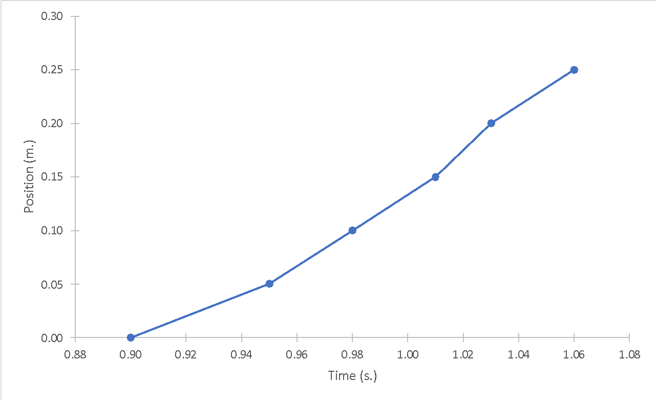
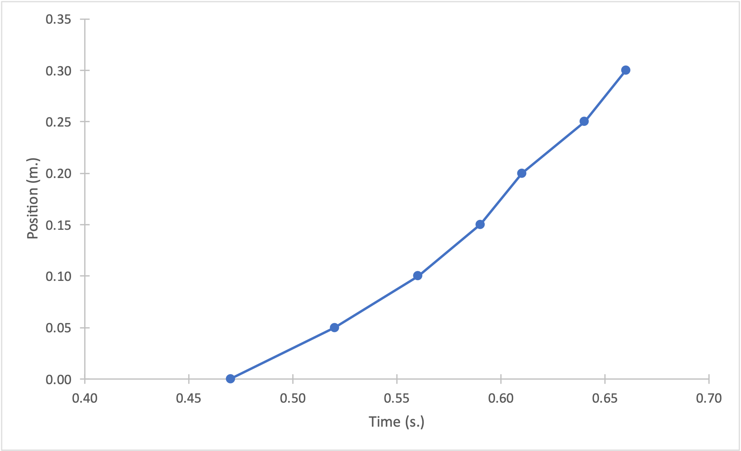
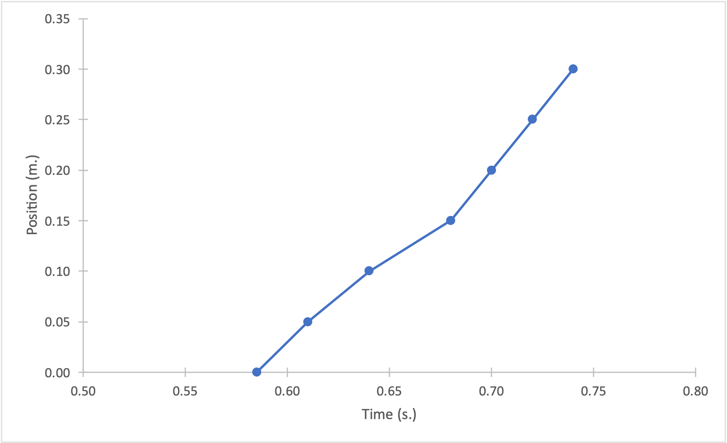
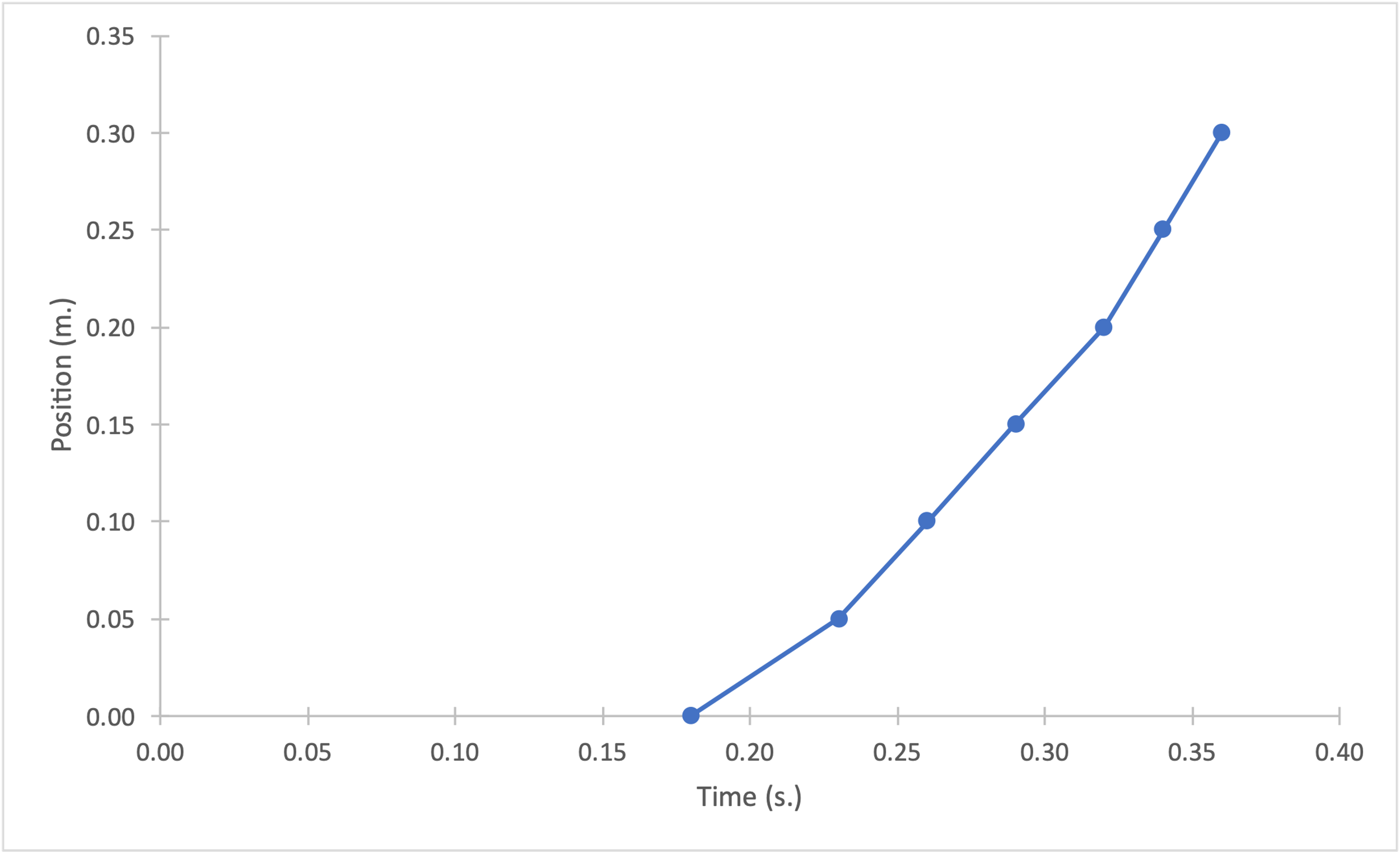
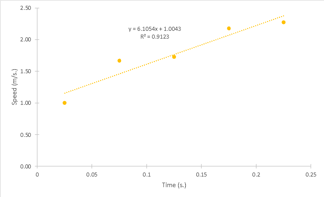
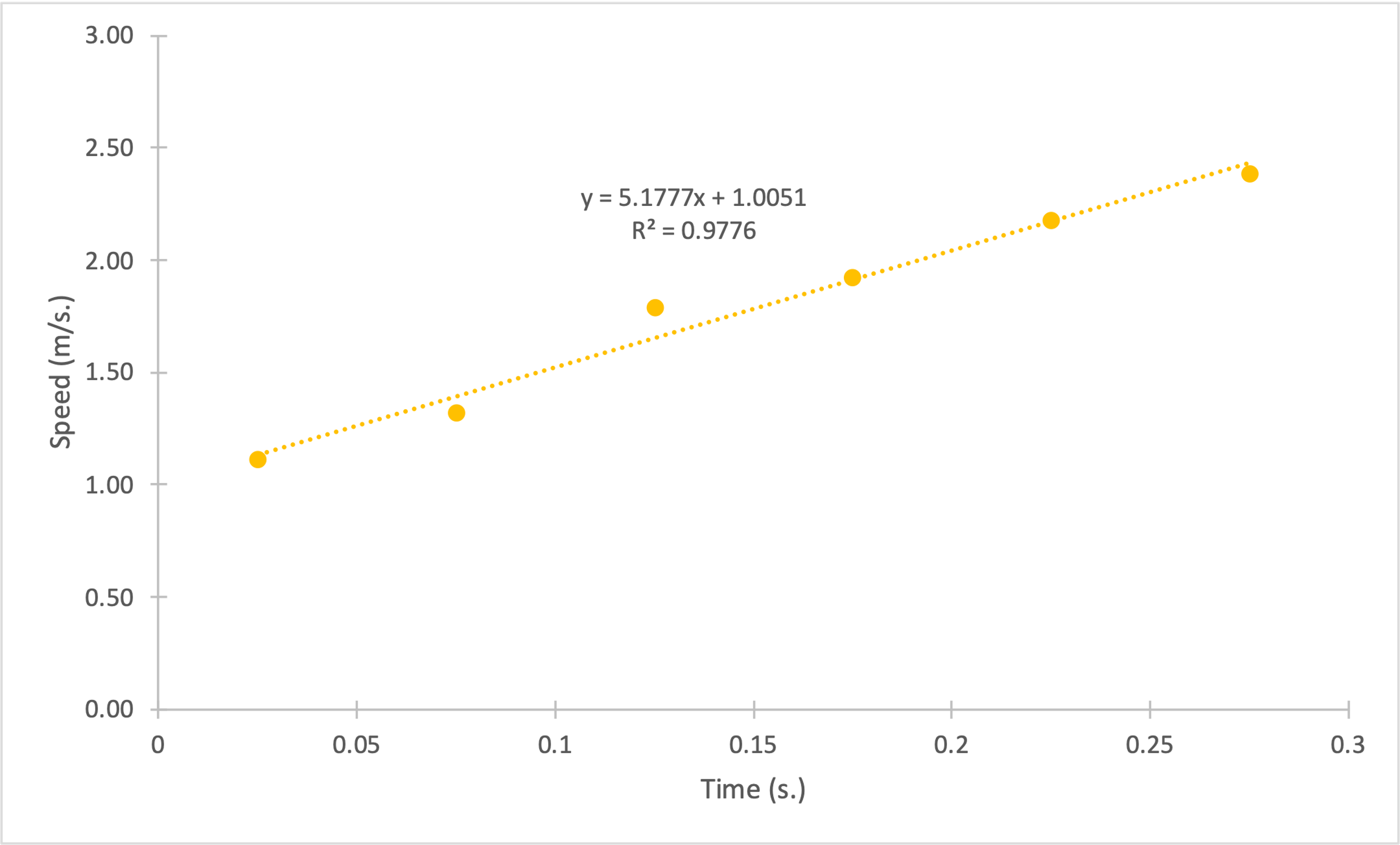
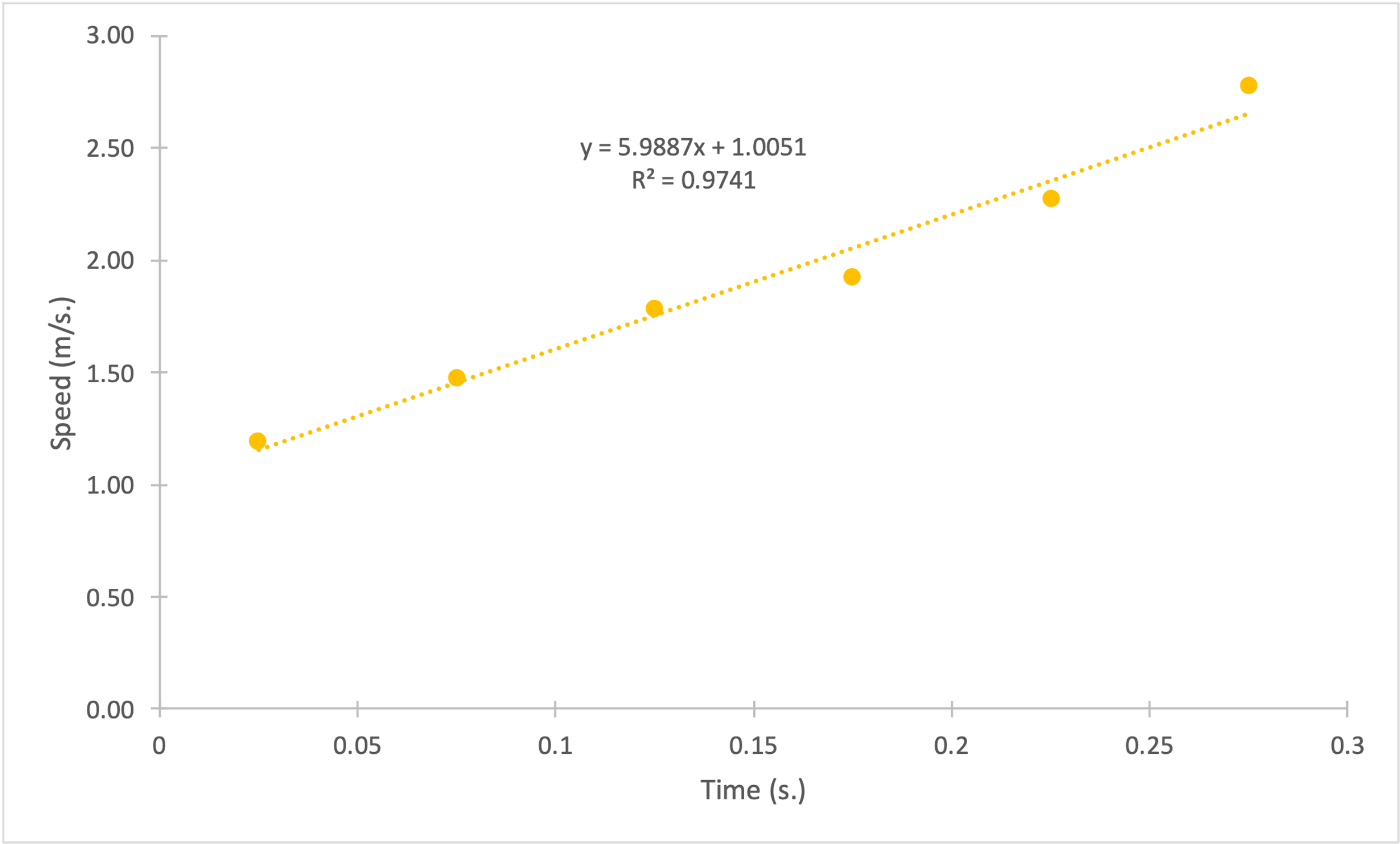
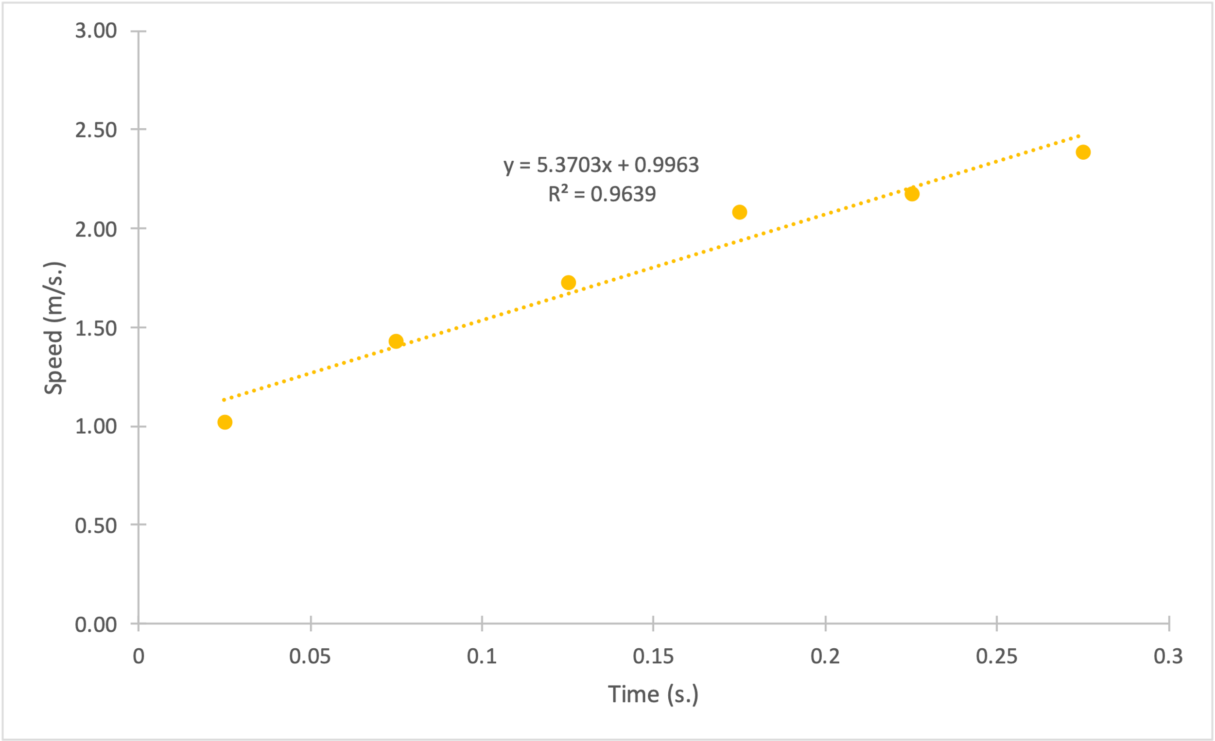
Figures 1-4 show plots of position (in m.) versus time (in s.) for each of the four launches. Strictly speaking, these data sets do not reflect perfectly linear trends for the dependencies, and thus, position as a function of time was not strictly linear. On the contrary, the plot of instantaneous velocity (in m/s) versus time (in s.) for each of the four cases could be classified as linear, which was clear, among other things, from the metrics of the linear regression equation.

Figures 5-8 show linear trend plots for the distribution of instantaneous velocity as a function of time for four falling objects. The acceptability of the linear model is determined by the coefficients of determination: the lowest value of this coefficient for the four objects is 0.9123, which is still quite high (Bloomenthal, 2021). In other words, it follows that the regression models cover more than 90% of the velocity variance for each of the distributions. In addition, we can infer the slope from the plots: the slope coefficient is equal to the free-fall acceleration for each case. We can see that this coefficient varies from 5.17 to 6.10 m/s², which differs from the reference value of 9.81 m/s².

Conclusion

This laboratory work has shown that it is possible to determine the free-fall acceleration by plotting a free-falling object. It was shown that the instantaneous velocity could be considered as a linear function of time. The calculated accelerations differed from the known value, which could be due to measurement uncertainties, errors, and measurement errors in the results. It is worth specifying that regression models were valuable tools for studying the dynamics of free-fall. However, the physical meaning of the y-intercept was absent for them since it defined a nonzero velocity at zero time.

Reference

Bloomenthal, A. (2021). Coefficient of determination. Investopedia. Web.