Introduction
Regression analysis is a statistical tool that is used to develop approximate linear relationships among various variables. Regression analysis formulates an association between several variables. When coming up with the model, it is necessary to separate between dependent and independent variables. Multiple regression analysis focuses on the regression between the dependent variable and several explanatory variables. The paper carries out a multiple regression analysis between the average free-flow speed (kph) and several explanatory variables such as the proportion of heavy vehicles, bendiness measure (degrees turned through per km), visibility, carriageway width (m), hard strip width (m), verge width (m), number of junctions per km and hilliness measure (meters of rising or fall per km).
Scatter diagram
A scatter diagram is a graph that plots two related variables on a Cartesian plane. The independent variable is plotted on the x-axis while the dependent variable is on the y-axis. In this case, the average free-flow speed (kph) is plotted on the y-axis while the other explanatory variables will be plotted on the x-axis. Scatter diagram tries to establish if there exists a linear relationship between two variables plotted on the diagram. This can be observed by looking at the trend of the scatter plots.
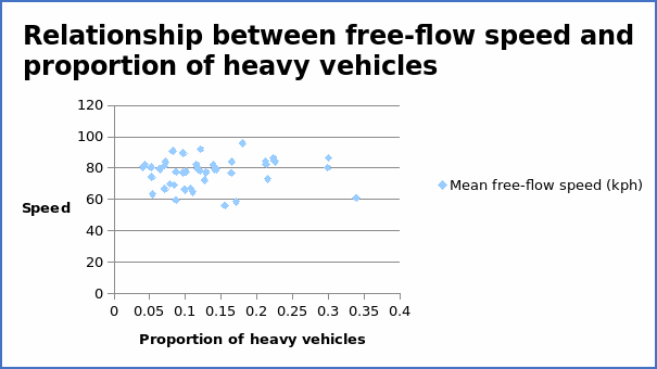
The correlation coefficient = 0.070015.
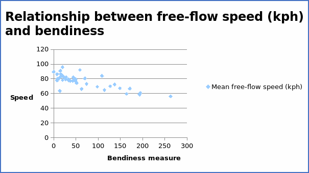
The correlation coefficient = -0.77625.
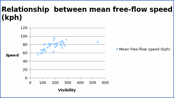
The correlation coefficient = 0.59998.
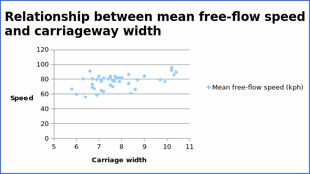
The correlation coefficient = 0.504263.
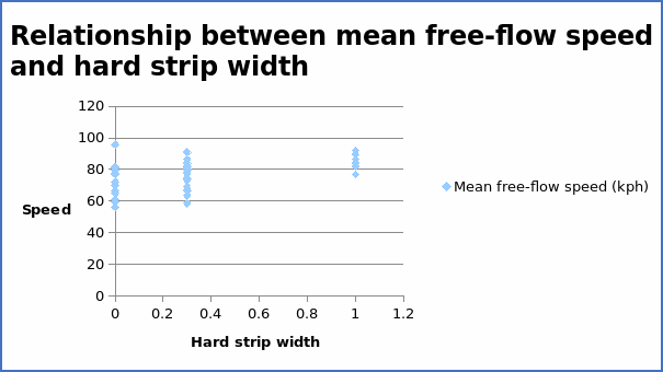
The correlation coefficient = 0.45776.
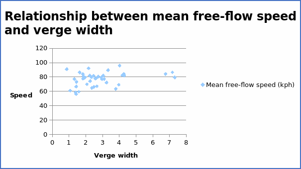
The correlation coefficient = 0.310631.
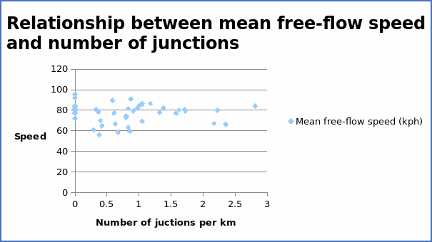
The correlation coefficient = -0.05523
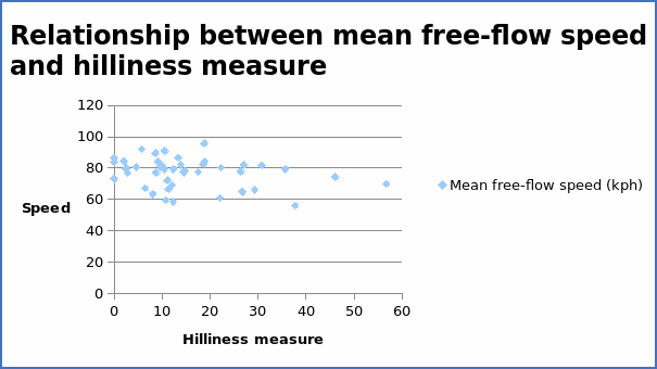
The correlation coefficient = -0.26919.
Points on the scatter diagram for the various diagrams slope in different directions. The table below summarizes the correlation coefficient for the various explanatory variables.
From the summary above, the visibility has the highest positive correlation coefficient of 0.59998. This implies that visibility will contribute by a large extent to increase in speed. On the other hand, bendiness has the highest negative correlation coefficient (-0.77625).
Simple regression analysis of speed and bendiness
The dependent variable is the mean free-flow speed, while the independent variable is the bendiness.
The regression line will take the form Y = b0 + b1X
Y = Mean free flow speed
X = Bendiness (degrees turned through per km)
The theoretical expectations are b0 can take any value and b1 < 0 (negative).
Regression Results
From the above table, the regression equation can be written as Y = 84.45057 – 0.11647X. The intercept value of 84.45057 denotes other variables that affect the average free-flow speed but are not included in the modelling. The coefficient value of -0.11647 implies that as bendiness increases by one unit, the average free-flow speed decreases by 0.11647 units. When the regression equation is compared with the scatter diagram, there is an indication of consistency. The graph of average free-flow speed (kph) and bendiness shows a downward trend with a correlation coefficient of -0.77625. The regression equation above also yields a negative slope. Thus, it is clear that the regression equation is sensible.
Evaluation of regression model
Evaluation of the regression model can be done by testing the statistical significance of the variables. Testing statistical significance shows whether the explanatory variable is a significant determinant of average free-flow speed. A two-tailed t-test is carried out at a 95% level of confidence.
Null hypothesis: Ho: bi = 0
Alternative hypothesis: Ho: bi ≠ 0
The null hypothesis implies that the variables are not significant determinants of demand. The alternative hypothesis implies that variables are a significant determinant of demand. From the table above, the values of t – calculated are greater than the values of t – tabulated. Therefore, the null hypothesis will be rejected, and this implies that bendiness is a significant determinant of the speed. Thus, it is statistically significant at the 95% level of significance. The value of the intercept is not relevant when testing the significance of the regression variables. Since the explanatory variable is statistically significant, it implies that the regression line can be used for prediction.
R-square value
The value of R2 is 60.26%. It explains 60.26% of the variation in free-flow speed. It is an indication of a strong explanatory variable. Also, the value of adjusted R2 is low at 59.26%. The value of R2 can be improved on by adding more variables in the regression model.
Analysis of variance
From the table, it is clear that the explained sum of squares (60.26%) is equal to the value of R2 discussed above (60.26%).
Unusual observations
Some of the unusual observations are summarized in the table below.
There are four outliers in the regression equation. Removal of these points will improve the regression line.
Simple regression analysis of speed and visibility
The dependent variable is the mean free-flow speed while the independent variable is the visibility.
The regression line will take a linear form Y = b0 + b1X
Y = Mean free flow speed
X = Visibility
The theoretical expectations are b0 can take any value and b1 > 0 (positive).
Regression Results
From the above table, the regression equation can be written as Y = 64.42415 + 0.067293X. The coefficient value of 0.067293 implies that if visibility increases by one unit, the average free-flow speed will also increase by 0.06793 units. The positive value of the coefficient implies a positive relationship between the variables. When the regression equation is compared with the scatter diagram, there is an indication of consistency. The graph of average free-flow speed (kph) and visibility shows a positive trend with a correlation coefficient of 0.59998. The regression equation above also yields a positive slope. Thus, it is clear that the regression equation is sensible.
Evaluation of regression model
A two-tailed t-test is carried out at a 95% level of confidence to test the significance of the variables
Null hypothesis: Ho: bi = 0
Alternative hypothesis: Ho: bi ≠ 0
From the table above, the values of t – calculated are greater than the values of t – tabulated. Therefore, the null hypothesis will be rejected, and this implies that visibility is a significant determinant of the explanatory variable (average free-flow speed). Thus, visibility is statistically significant at the 95% level of significance. The value of the intercept is not relevant when testing the significance of the regression variables.
R-square value
The value of R2 is 36.00%. This implies that visibility explains only 40% of the variation in free-flow speed. It is an indication of a weak explanatory variable. Also, the value of adjusted R2 is low at 34.39%. The value of R2 can be improved on by adding more variables in the regression model.
Analysis of variance
From the table, it is clear that the explained sum of squares (36.00%) is equal to the value of R2 discussed above (36.00%).
Unusual observations
Visibility is commonly known to be a significant determinant of average flow speed. The result above is contrary to the common knowledge as indicated as the weak regression line. The regression line has several outliers, and this contributes to the weak model. Removal of the outliers will strengthen the regression equation.
Simple regression analysis of speed and hilliness
The dependent variable is the mean free-flow speed while the independent variable is the hilliness
The regression line will take the form Y = b0 + b1X
Y = Mean free-flow speed
X = Hilliness
The theoretical expectations are b0 can take any value and b1 < 0 (negative).
Regression Results
From the above table, the regression equation can be written as Y = 80.1933 – 0.20343X. The coefficient value of -0.20343 implies that if hilliness increases by one unit, the average free-flow speed decrease by 0.20343 units. The positive value of the coefficient implies a positive relationship between the variables. When the regression equation is compared with the scatter diagram above, there is an indication of consistency. The graph of average free-flow speed (kph) and hilliness shows a negative trend with a correlation coefficient of -0.26919. The regression equation above also yields a negative slope. Thus, it is clear that the regression equation is sensible.
Evaluation of regression model
A two-tailed t-test is carried out at a 95% level of confidence to test the significance of the variables
Null hypothesis: Ho: bi = 0
Alternative hypothesis: Ho: bi ≠ 0
The table below summarizes the results of the t-tests.
From the table above, the value of t – calculated is less than the values of t – tabulated for visibility. Therefore, the null hypothesis will not be rejected, and this implies that hilliness is not a significant determinant of the explanatory variable (average free-flow speed). Thus, hilliness is not statistically significant at the 95% level of significance. The regression model shows that the slope is weak and cannot explain the variations in speed.
R-square value
The value of R2 is 7.25%. This implies that hilliness explains only 7.25% of the variation in free-flow speed. It is an indication of a weak explanatory variable. Also, the value of adjusted R2 is low at 4.92%. The value of R2 can be improved on by adding more variables in the regression model.
Analysis of variance
The table below summarizes the analysis of variance.
The RSS is greater than ESS by a large margin. From the table, the explained sum of squares (7.25%) is equal to the value of R2 discussed above (7.25%). It shows that the model is irrelevant in determining the variations of speed. In real life, technology has lead to innovation of high power car such that hilliness cannot cause a reduction of speed.
Unusual observations
Over 90% of the observations are outliers. Thus, the removal of all these points would amount to eliminating the variable from the regression model.
Multiple regression regression results
The regression line will take the form Y = a0 + a1X1 + a2X2 + a3X3 + a4X4 + a5X5 + a6X6 + a7X7 + a8X8. This section will summarize the results of various iterations of multiple regression analysis.
First regression – speed and proportion of heavy vehicles
The variable is not statistically significant at the 95% level of confidence.
Second regression – speed and proportion of heavy vehicles and bendiness
The additional variable is statistically significant, and it improves the value of R2 to 61.36%.
Third regression – speed and proportion of heavy vehicles, bendiness and visibility
The additional variable improves the value of R2 to 64.85%
Fourth regression – speed and proportion of heavy vehicles, bendiness, visibility and carriageway width
The additional value reduces the values of t – computed, but it increases the R2. It is not statistically significant.
Fifth regression – speed and proportion of heavy vehicles, bendiness, visibility, carriageway width and hard strip width
The additional value reduces the values of t – computed, but it increases the R2. It is not statistically significant.
Sixth regression – speed and proportion of heavy vehicles, bendiness, visibility, carriageway width, hard strip width and verge width
The additional value increases the values of t – computed for other variables, and it also increases the R2. It is not statistically significant.
Seventh regression – speed and proportion of heavy vehicles, bendiness, visibility, carriageway width, hard strip width, verge width and number of junctions
The additional value reduces the values of t – computed for other variables, and it increases the R2. It is not statistically significant.
Eighth regression – speed and proportion of heavy vehicles, bendiness, visibility, carriageway width, hard strip width, verge width, number of junctions and hilliness
The additional value reduces the values of t – computed for other variables, and it also increases the R2. It is not statistically significant.
From the regression analysis above, only the variables are significant, and they lead to an increase in values of t – calculated these are, bendiness, visibility, and hardship strip. The variables increase the values of t – computed. The variables also increase the amount of R2 by a large margin. All the other variables should be dropped from the regression model.
Alternative models
There are several modelling techniques that can be used apart from the regression model. Some of them are polynomial models, logit and probit, among others. An example of the polynomial regression is shown below.
Y = a0 + a1X1 + a2X2 + a3X32 + a4X4 + a5X5 + a6X6 + a7X72 + a8X8.
The results are shown above.
The model improves the value of R2 to 70.01%.