Introduction
Sensitivity analysis and linear programming are important statistical tools of analysis when faced with the challenge of making a decision against series of constraints in business. As referred to as linear optimization, linear programming is applied in attempting to get the best outcome from series of other outcomes with a linear relationship with an intention of achieving an optimal outcome. On the other hand, sensitivity analysis is used in establishing the level of uncertainty in an output that is numerical or non-numerical by apportioning different units of uncertainties in the inputs used to generate the output.
These two statistical tools are significant in testing robustness of different results, establishing optimal outcome, and parameters of input-output relationship. This chapter explores different elements of sensitivity analysis and linear programming such as settings, methodology, application, and integration. Besides, the chapter applies different scientific reasoning to explore the details in context, modeling, and solution as applied in linear programming and sensitivity analysis. In addition, the chapter summarizes the general use of these tools in making scientific sense when faced with different constraints that require integration of different inputs to derive an optimal output with the least possible cost implication at the maximum benefit level.
Sensitivity Analysis
Sensitivity analysis is basically a mathematical model annotated by equations, parameters, and input variables with the intension of classifying the progression being investigated. Sensitivity analysis might be applied in generating finite element, economic, and climate models in different fields of application (Cacuci, 2011). Since such models are very complex due to series of interacting inputs and outputs, there is need to generate sensible understanding of the phenomenon being investigated.
Therefore, there is need to establish the uncertainty, measurement error, and confidence level in order to create the intrinsic system variability. Sensitivity analysis as a modeling practice comes in hand in solving the above puzzles by quantifying uncertainty level, evaluation the degree to which every input contributes to uncertainty in the output, and ranking the inputs in an appropriate order to establish the potential uncertainty in the output. Specifically, when the mathematical model has many variables in the form of inputs, sensitivity analysis becomes an important instrument for quality assurance and model building (O’Hagan, 2006).
The method applied in sensitivity analysis is dependent on the digits of problem settings and constraints. The sensitivity analysis is applied in modeling the computational expense, correlated outputs, non-linearity, model interactions, multiple outputs, and given data. Under computational expense, sensitivity analysis is applied by running this model several times within the preset sample base by using screening methods and emulators. Under correlated outputs, sensitivity analysis assumes complete independence between inputs in order to establish the correlation. The same approach is applied in other methods with slight variations in correlation different variables in discrete optimization (Cacuci, 2011).
The core methodology of carrying out sensitivity analysis is similar, irrespective of the number input variables and approach adopted. The guideline for carrying out sensitivity analysis encompasses four steps. The first step is quantification of the uncertainty within each input in terms of probability and range. The second step is identification of the output model that is supposed to be analyzed, which must be directly related to the problem to be solved. The third step is running the model severally via experimental designs that are determined by input uncertainty and chosen method. The last stage is using the mode output results to compute the sensitivity interest (Saltelli, 2009).
There are several methods of carrying out sensitivity analysis, depending on the number of inputs and outputs to be calculated. Among the notable methods of carrying out sensitivity analysis include One-at-a-time (OAT), scatter plots, regression analysis, variance-based method, and screening. Under the OAT method, the strategy is to examine how variation in a factor at a time affects the output generated. For instance, a single input variable is moved while maintaining other normal variables at the baseline. The moved variable is then returned at the baseline after which another variable at the baseline is moved. The process is repeated depending on the number of variable inputs (Saltelli, 2009).
The degree of sensitivity is them measured by examining the variations in the output when each of the input variables are moved and replaced at the baseline through linear regression or partial derivatives. Through series of changes applied to each input variable, it is possible to maintain other variables as constant or fixed at the baseline to ensure than variations in the output is equitable to change in a single input variable. Under the scatter plot method, a plot is drawn for different scatter spots of the resulting output variable as a function of the input variables through a random sampling model to ensure that arbitrary data points can be compared in terms of visible sensitivity variation from the plot (Cacuci, 2011).
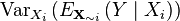 function. In this case, Var denotes the variance while E denotes the expected value. Besides, X~I represents all sets of input variables with an exception of Xi (Saltelli, 2009).
Example
In the Dubai car industry, the choice of car being purchased by customer is assumed to be dependent on the variables of price and per mileage consumption of different car models in the market. A set of data was collected on the trend to represent the purchasing behavior of customers within the Dubai car industry. The information was generated in a table to rank ten pairs of observations for x and y where x=Km’000 and Y=AED ‘000. The data was then plotted in a graph below to indicate the results.
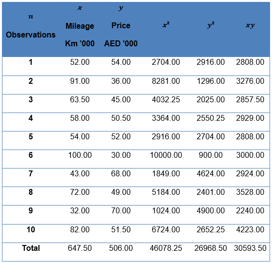
In order to carry out sensitivity analysis, there is need to establish the input variables (mile and price) and output (preferred car model). The above data can be used to generate a scatter graph by randomly picking values and plotting against mileage and price as indicated in the table below.
 . Apparently, the choice of car model is highly sensitive to the mileage of the vehicle and price.
Linear Programming
Linear programming is a method of linear objective function optimization within the constraints of linear equality and inequality. The objective function of a linear equation is defined on the polyhedron of the real value (Bernd, 2006). The connation of a linear problem is represented as;
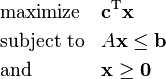
In the above function, x is the vector of the variables that are supposed to be resolved. The letters c and d represent the coefficient vectors while letter A represents the coefficient matrix. Lastly,
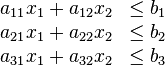
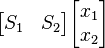
 represents the transpose matrix. In application, the function might be minimized or maximized into an objective function where the inequalities are modified onto comparable vectors with similar dimensions. Application of linear programming occurs in many fields such as economics, business, and engineering among others to optimize an outcome from a series of other outcomes that can be generated. For instance, in solving a multi-commodity problem in the business environment, linear programming becomes instrumental in generating a series of algorithms from which an optimal solution can derived, with the primary intension of maximizing the returns at the least possible cost implication (Dmitris & Padberg, 2010). The standard linear function is represented as follows. When the linear function is to be maximized, it takes the form of
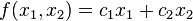
Therefore, the non-negative variables will be;

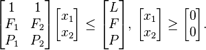
In order to present the linear problem in a matrix form, it will take the functional representation as;

Illustration of application of linear programming
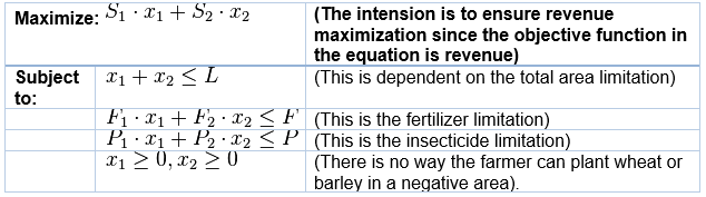
Suppose a farmer has L km2 of land where intends to plant either barley and wheat or both crops in the same land. The fertilizer that the farmer can access is limited to F kilograms. The insecticide is also limited to just P kilograms. For the wheat to be planted per square kilometer, the farmer will use F1 fertilizer kilos and P1 insecticide kilos. On the other hand, for the barley to be planted per square kilometer, the farmer will use F2 fertilizer kilos and P2 insecticide kilos. Further, the price of selling wheat grown per square kilometer is represented by S1 while the price of selling barley grown per square kilometer is represented by S2. The space of land where wheat and barley are planted is represented by X1 and X2, correspondingly. Therefore, in order to maximize yield, which is the same as profits for the farmer, there is need to choose the optimal X1 and X2 values. In order to solve the above problem using linear programming, the first step would be creating standardized linear function that accommodates all the constraints (Bernd, 2006). This is calculated below.
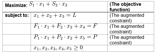
From the above constraints and function, the linear matrix takes the form of minimizing
subjected to
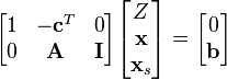
In order to simply the above matrix, there is need to create an augmented form of the function to apply simplex algorithm by introducing a non-negative variables to substitute constraint inequalities with constraint equalities as presented in the function below in the form;
Maximize Z:
x, xs ≥ 0
In the above augmented function, xs represents the new slack variable introduced in the original function while Z represents the variable which is supposed to be maximized. When the slack variables are introduced, the linear function will take the form;
In the above functions, the slack variables are represented by
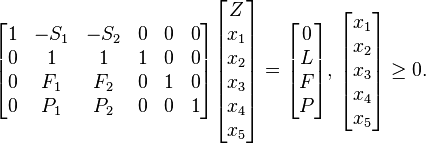
 , which connotes the area not used, fertilizer not used, and insecticide not used by the farmer.
In the matrix form, the function will can be represented as;
Maximize Z:
When there is a definite solution as is the case with the above example, the optimal output is derived from the linear objective function at the edge of different optimal set levels through maximum principle (Schrijver, 2009). In complex linear problems, optimal solutions can be obtained by using other algorithms such as simplex, criss-cross, ellipsoid, projective, and path-following forms. However, most of these algorithms are preprogrammed in different software for generating optimal output when different input variables are fed in the software sheet (Dmitris & Padberg, 2010).
Real example
A trader intends to buy some cabinets denoted by X and Y. The trader is aware that the cost of cabinet X is $10 and can be fitted in a floor space of 6 square feet to hold files that are 8 cubic feet in depth. The cost of a unit of cabinet Y on the other hand is $20 and needs an office space of 8 square feet in order to hold files that have a depth of 12 cubic feet. The trader has $140 to acquire cabinet X and Y to fit the office space that can accommodate cabinets within 72 square feet. In order to determine the number of each model of cabinet to be purchased to offer maximum storage capacity, the variables to consider are x; number of X model cabinets, and y; number of Y cabinets to purchase. Obviously, y > 0 and x > 0 since there is no way the trader can make negative purchase of cabinet X and cabinet Y. The next step is to take into account the floor space and costs at maximum storage capacity. In this case, the floor space and costs are the constraints with the volume being the optimization equation as summarized below.
- Cost: 10x + 20y < 140, or y < – (1/2) x + 7
- space: 6x + 8y < 72, or y < – (3/4) x + 9
- volume: V = 8x + 12y
The equation can be plotted in the linear graph inclusive of the two constraints as indicated below.
From the above graph, when the corner points are tested at (12, 0), (0, 7), and (8, 3), the maximum volume that can be obtained is 100 cubic feet through purchasing 3 units of cabinet Y and 8 units of cabinet X.
Conclusion
Linear programming and sensitivity analysis are important statistical tools for making decision based on examining the interaction between different variable inputs to generate ideal output. Specifically, linear programming is significant in ensuring that optimal output is achieved by subjecting different input variables and constraints for the best solution at the least cost. On the other hand, sensitivity analysis measures the relationship between output and input, in terms of how a unit change in each unit input can affect the output generated.
Reference List
Bernd, G. (2006) Understanding and using linear programming. Berlin: Springer. Web.
Cacuci, D. (2011) Sensitivity and uncertainty analysis: Theory. New York: Chapman & Hall. Web.
Dmitris, A. & Padberg, P. (2010) Linear optimization and extensions: Problems and solutions. New York: Springer-Verlag. Web.
O’Hagan, A. (2006) Uncertain judgments: Eliciting experts’ probabilities. New York: Wiley Chichester. Web.
Saltelli, A. (2009) How to avoid a perfunctory sensitivity analysis. Environmental Modeling and Software Journal. 25 (4). p. 1508–1517. Web.
Schrijver, A. (2009) Combinatorial optimization: Polyhedra and efficiency. Berlin: Springer. Web.