Introduction
There is no doubt that statistics is a multifaceted concept with a myriad of applications; currently, everything ranging from sociology, science, business to mention but a few in one way or another incorporate statistics in their day-to-day activities. With this in mind, it is worth noting that several statistical analyses are having varied applications and need to be mastered. This paper exclusively deals with the analysis of multivariate data. Multivariate data analysis is twofold, first, it is a scientific field that indulges in multivariate observation of a given phenomenon and secondly, it is a mathematical aspect that deals with the development of models that describe the relationship of a given data variable (Long, 1997).
The main reason for this analysis is to establish the relationships between the variables in a data set. This will utilize some of the key tools such as regression and correlation. To accomplish this, the income. sav the dataset from session 8 will be utilized. In the first section, correlation analysis will be carried out to establish the relationship between income and class. In the second part, a further analysis terms logistic regression analysis will be carried out to find out how the above mention relationship varies when other co-factors are brought in simultaneously. With this, a prediction equation is clearly stated.
Correlation analysis
In the strictest sense, correlation is a statistical analysis that aims in exploring the relationship between two numerical variables. When such an analysis is executed, the results help researchers determine three major issues; the existence of a linear or a straight-line relationship, the strength of the association or link, and lastly the direction of the association whether it is positive or negative (Long, 1997). There are normally two approaches to accomplish this; using Pearson’s correlation or Spearman’s Rho. The former is applicable when dealing with two numerical variables that are normally distributed and the latter is applied when dealing with one or all the variables are in the ordinal scale or when one numerical variable neither is nor normally distributed.
Income is treated as the dependent variable while social class is the independent variable. The statistical setup is based on the assumption that social class can be used to predict an individual’s income (Bryman & Cramer, 1999). Other than identifying whether social status can be used to evaluate an individual’s income, the statistical evaluation will also be used to establish the kind of relationship and whether there exists any recognizable trend in relation. Correlation analysis is used to establish whether there exists any relationship between the dependent and the independent variable. The following table shows the statistical output for correlation analysis between gross weekly individual income and social class.
Correlation coefficient
The correlation coefficient r is used in the measurement of the linear relationship between the two variables, namely, an individual’s gross income and social class. This is also known as the Pearson product-moment correlation coefficient. Its value is expected to lie within the range defined by the equation below: -1 ≤ r ≤ + 1.
A value close to 0 indicates little correlation. The further from zero the value is, the more correlation is considered to exist. Higher positive correlation values show that the dependent variables would exhibit a direct proportionality relationship with the independent variable. In this case, this would be interpreted to mean that an increase in the Social class category would result in increased income estimates (Achen, 1982). Increased negative correlation values show that change in the independent variable would result in a corresponding inverse change in the dependent variable. In this case, a decline in social class would amount to a decline in individual gross income. This is best summarized by the statements hereafter.
Consider the variables, social class, and individual gross income:
- When r = 1, then social class and individual gross income exhibit perfect correlation. The prospective values of social class and individual gross income are in a straight line with a slope in the (social class, individual gross income) plane.
- When r = 0, social class and individual gross income are non-correlated. They lack an apparent linear relationship. However, this does fully indicate that social class and individual gross income have statistical independence.
- When r = -1, social class and individual gross income bear a perfect negative correlation. The prospective values of social class and individual gross income are in a straight line with the slope in the (social class, individual gross income) plane.
Table 1 Correlations analysis between Social class and individual income (Equal Data).
It is worth noting that the results of Spearman’s correlation which was aimed at establishing the relationship between social class and individual income show that the relationship is significant but negative and moderate (Rho=-0.560, p=0.000). This thus confirms that an individual’s income decreases along with the presumed social class decline (Figure 1)
Logistic regression analysis
According to Chao-Ying et al., 2002 it is worth remembering from the onset that not all socio-economic variables are continuous and interval. In such a situation, the variables are categorical and dichotomous. For this reason, it will be irrational to carry out multiple linear regression analyses. Thus this is where logistic regression analysis comes into play as it perfectly analyzes categorical dependent variables.
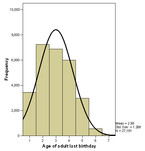
For this section, a logistic regression analysis will be conducted with rich or poor as being the variable being predicted. The three predictor variables being used include social class, gender, and age of the respondents. Age is an interval level variable and gender is a dichotomous or dummy-coded nominal variable; for these reasons, it is thus evident that the two variables meet the requirement of logistic regression analysis.
Similarly, the variable rich or poor is an ordinal level variable, and following the convention of handling such a kind of measurement as being a metric one, then one can conduct logistic regression analysis. Having in mind that the analysis is not executable when dealing with categorical variables such as social class, there is a need to first convert them into a series of dummy variables which is accomplished automatically using SPSS. Tables 2 to 5 show the frequencies distribution of the three major independent variables.
From the table, there are 45202 cases included plus those that might be later established to be outliers or influential cases. The dependent variable is encoded Poor=0 and Rich= 1. Regarding sex/gender males are encoded 0 and females 1 (Table 7).
Block 1: Method Enter
Adding gender to the model reduces -2 log-likelihood by 3282.669. The p-value is 0.000 which is less than the significance level set at 0.05 this guides the conclusion that when sex or gender is added to the statistical significance is realized hence it explains variation in being ‘Rich’ or ‘Poor’ (Chao-ying et al, 2002)


From the table above the estimated model is: Rich or Poor=-0.788+ -1.416Sex (1)
Since male was coded as 0 and female as 1; then Rich or Poor =-0.788+ -1.416 Female
The Exp (B) depicts the relative odds and indicates that females are 0.243 times to be richer than males. When a second variable age is introduced, it reduces the -2 log-likelihood by 508.741 on 1 DF. Thus the model when having two variables sex and age collectively reduces the -2 log-likelihood by 3791.410. Of the two variables, it is apparent that gender/sex has more explanatory power than age. From the summary model, sex/gender and age explain between 8.0 % and 12.7% of the variation in being Rich or Poor.
Block 2: Method=Enter
Considering the two variables the models equation then becomes;
Logit (Poor or Rich) =1.196+ (-1.417) female+ (-0.158) age (Table 18)
Age is statistically significant since the p-value is 0 and is thus smaller than the alpha set at 0.05. The Exp (B) is 0.854 which when interpreted means for each year difference in age an individual is 0.854 more likely to be rich when sex/gender is factored in the model. A general notion here is that whenever one is older, he/she is either richer or poorer depending on other variables (Hosmer & Lemeshow, 2000).
Social class, a third variable is to be added to the model as Block 3. It is worth remembering that social class is a categorical variable just as gender/sex was. There is thus a need to set up dummy variables where the first category is the reference one (Achen, 1982).
Block 3: Method=Enter
Social class is statistically significant in the model (Chi square=14326.910, DF=9, p=0.000)
From model summary table 19 the three variations caused as a result of age, gender, and social class range between 27.2% and 43.0%.
After considering all the three variables; age, gender, and social class the model for prediction then becomes;
Logit(Rich)=0.744+[-1.303gender(1)]+0.80age+[-0.609 social class(1)]+[-2.043social class(2)] (Table 21)
This can be translated as follows;
Logit (Rich) =0.744+ [-1.303female] +0.80age+ [-0.609professionals] + [-2.043unknown]
Social class(1) corresponding to a professional has Exp(B) of 0.544 depicts that a person who is a professional is only 0.544 times much less to be rich/poor than an individual who in managerial or technical having factored in gender and age. Calculating an inverse of Exp (B) in this case 1/0.544 = 1.84 means that an individual who is in managerial or technical class is 1.84 times more likely to be rich than a professional (Hosmer & Lemeshow, 2000).
Conclusion
From the analysis of multivariate variables using regression and analysis, insight can be gained on the relationship between variables. In this case, there was a relationship between social class and individual income in terms of weeks being considered as [Equal Data]. However, it was moderate negative and significant (Rho=-0.560, p=0.000). Concerning logistic regression analysis, it is evident that all the three variables (age, sex/gender, and social class) are significant in predicting the dependent variable Rich/Poor.
References
Achen, C. (1982). Interpreting and Using Regression. London: Sage.
Bryman, A. & Cramer, D. (1999). “Quantitative Data Analysis with SPSS for Windows: A Guide for Social Scientists”, Chapters 9 and 10. Journal of Mathematical & Statistical Psychology, 57(1), pp.173-181.
Chao-ying J., Kuk, L & Ingersoll, G. (2002). “An Introduction to Logistic Regression Analysis and Reporting” The Journal of Educational Research, Vol. 96 No. 1 pp 1-13.
Hosmer, D. & Lemeshow, S. (2000). Applied Logistic Regression. New York: John Wiley & Sons, Inc.
Long, J. (1997). Regression Models for Categorical and Limited Dependent Variables. Thousand Oaks, CA: Sage Publications.
Appendices
Table 2 Social Class distribution frequency.
Table 3 Sex distribution frequency.
Table 4 Age of adult last birthday.
Table 5 Rich (top 5th of the population).