Two-Way Factorial Anova Analysis

Introduction

This paper reports the results of an analysis of data using a two-way factorial ANOVA. The data set is briefly described; the assumptions for the factorial ANOVA are named and tested; the research question, hypotheses, and alpha level are articulated; and the results of the analysis are provided. Finally, some strengths and limitations of the factorial ANOVA are briefly discussed.

Data File Description

The caffeineexercisehr.sav data set contains the results of a hypothetical study of the impact of caffeine and exercise on heart rates (Warner, 2013, p. 544). Thus, the factors are caffeine (1=no caffeine, 2=150 mg of caffeine) and exercise (1 = no exercise, 2 = half an hour of exercise), and the outcome is heart rate (beats per minute) (Warner, 2013, p. 544). The independent variables are both dichotomous, whereas the dependent variable is interval/ratio. The sample size N=16.

Testing Assumptions

The assumptions for a factorial ANOVA are as follows (Warner, 2013, pp. 506-507):

1. the dependent variable is quantitative;
2. the dependent variable is approximately normally distributed;
3. the independent variables are independent of each other, and the cases in the data set are pairwise independent;
4. homogeneity of variances of the scores of the dependent variable in different groups;
5. no extreme outliers in the dependent variable.

Assumptions 1, 2, and 5

The dependent variable is quantitative (thus, assumption 1 is met).

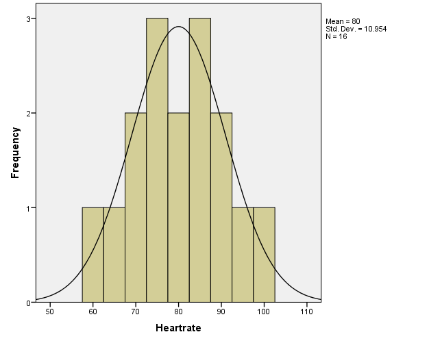
Figure 1 above shows the histogram for the dependent variable. It appears that the variable is approximately normally distributed (the assumption 2 is met). There are no outliers (assumption 5 is met).

Table 1. Descriptives for the heart rate variability.

Table 1 above shows the skewness and kurtosis for the dependent variable. The distribution of the variable is perfectly symmetrical around the mean (skewness=0), and slightly “flatter” than the normal distribution (kurtosis=-.491). Both values are ideal for analysis in respect of skewness and kurtosis (George & Mallery, 2016).

Assumptions 3 and 4

The factors do not depend on one another, and the observations are pairwise independent (because they are gathered from different participants), so the assumption 3 is met.

Table 2. The results of Levene’s test for homogeneity of variances across groups.

Table 2 above shows the results of Levene’s test of homoscedasticity of the scores of the dependent variable across groups. The test yielded F(3, 12)=.000, at p=1.0, which indicates that there are no significant differences in variances across groups. So, assumption 4 is met.

Therefore, all the assumptions for the factorial ANOVA are met.

Research Question, Hypothesis, and Alpha Level

The research question for the given data set that can be tested by the factorial ANOVA is as follows: “Do the intake of caffeine, exercise, and the interaction between the intake of caffeine and exercise predict heart rates of participants?” The null hypothesis for the first factor is as follows: “There is no significant difference in the means of heart rates between the group that took caffeine and the group that did not take caffeine.” The null hypothesis for the second factor is: “There is no significant difference in the means of heart rates between the group that exercised and the group that did not exercise.” The null hypothesis for the interaction is: “There are no significant differences in the means of heart rates between different caffeine×exercise groups.”

The alternative hypothesis for the first factor is: “There is a significant difference in the means of heart rates between the group that took caffeine and the group that did not take caffeine.” The alternative hypothesis for the second factor is: “There is a significant difference in the means of heart rates between the group that exercised and the group that did not exercise.” The alternative hypothesis for the interaction is: “There are significant differences in the means of heart rates between different caffeine×exercise groups.” The alpha level for this test will be α=.05, which is the standard level (Field, 2013), for no rationale for using any other alpha levels is known.

Interpretation

Means for the Dependent Variable

• The Appendix indicates that the grand mean for the heart rate variable was 80.0.
• The Appendix also shows that the mean heart rate for the group that did not take caffeine was 72.5, whereas the mean for the group that took caffeine was 87.5.
• The Appendix also demonstrates that the mean heart rate for the group that did not exercise was 75.0, whereas the mean for the group that exercised was 85.0.

Also, the Appendix shows that the mean heart rate for the group that did not take caffeine and did not exercise was 67.5, and for the group that did not take caffeine but exercised was 77.5; the mean heart rate for the group that took caffeine but did not exercise was 82.5, and for the group that took caffeine and exercised was 92.5.

Means Plot for the Dependent Variable

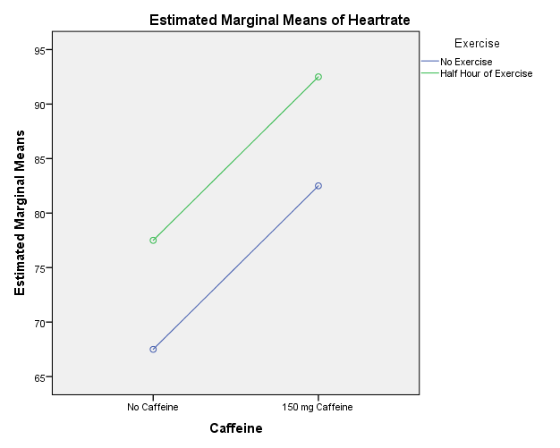
Figure 2 shows the estimated marginal means for the dependent variable. Each of the two factors increases the scores of the outcome. Thus, the main effects for each of the independent variables are that the heart rates of participants are increased. The statistical test below will check whether these main effects are significant.

It also can be seen that the two lines are parallel. Therefore, it appears that there is no interaction between the independent variables, for the effect of one factor on the outcome does not change depending on the other factor (Field, 2013).

Results of the Factorial ANOVA

Table 3. Results of the ANOVA test.

Therefore, Table 3 shows that there was a significant difference in the means of heart rate for the caffeine variable: F(1)=21.6, p=.001. The effect size η²=21.6/(21.6+12)=.64, which is large effect size.¹ The observed power is.989, so the odds of finding an existing effect was 98.9%, and the odds of making a type II error was 1.1% (Warner, 2013). Thus, the null hypothesis for the first factor was rejected; the evidence was found to support the corresponding alternative hypothesis.

There also was a significant difference in the means of heart rate for the exercise variable: F(1)=9.6, p=.009. The effect size η²=9.6/(9.6+12)=.444…, which is large effect size. The observed power was.811, so the odds of making a type II error were 1-.811=.189, or 18.9% (Warner, 2013). Therefore, the null hypothesis for the second factor was rejected; the evidence was found to support the respective alternative hypothesis.

The interaction caffeine×exercise was not significant: F(1)=0, p=1. The effect size η²=0/(0+12)=0, a zero effect size. ² The observed power was.05, so the odds of making a type II error were 1-.05=.95, or 95%. The null hypothesis for the interaction of factors was not rejected.

Conclusion

Therefore, a two-way factorial ANOVA was conducted to check whether the intake of caffeine, exercise, and the interaction between the intake of caffeine and exercise could predict heart rates of participants. It was discovered that both the intake of caffeine and the exercise could predict the heart rates of participants; the differences in the means in both cases were both statistically significant and of large magnitude (large effect size). However, there was no interaction between the factors (p=0, zero effect size).

The factorial ANOVA has several strengths; for example, it allows for examining differences in means of the outcome for each of several factors simultaneously, so there is no need to run separate tests; it is also virtually the only effective choice for exploring the results of an interaction (Warner, 2013). However, it also has its disadvantages; for instance, as a parametric test, it relies on certain assumptions (such as homoscedasticity in all the groups of the design) the violation of which can make the test considerably less reliable (Warner, 2013).

References

Field, A. (2013). Discovering statistics using IBM SPSS Statistics (4th ed.). Thousand Oaks, CA: SAGE Publications.

George, D., & Mallery, P. (2016). IBM SPSS Statistics 23 step by step: A simple guide and reference (14th ed.). New York, NY: Routledge.

Warner, R. M. (2013). Applied statistics: From bivariate through multivariate techniques (2nd ed.). Thousand Oaks, CA: SAGE Publications.

Appendix

Descriptive statistics for heart rate variable for different groups formed by caffeine and exercise variables:

Footnotes

1. According to Warner (2013), the effect size for a factor A as measured by η² can be calculated as follows: η²_A = (df_A * F_A) / ((df_A * F_A) + df_within), where df_within = ab(n-1),where a is the number of levels of factor A, b is the number of levels of factor B, n is the number of cases in each cell of the design.
2. According to Warner (2013), the effect size for the interaction A×B as measured by η² can be calculated as follows: η²_A = (df_A×B * F_A×B) / ((df_A×B * F_A×B) + df_within).