Introduction
This report analyzes the impact of the number of calls made by salespeople on sales. A sample of 100 data points, measuring weekly sales and the number of calls, serves as the basis for this report. Statistical data analysis was performed to assess the relationship between the number of calls and sales.
Initially, the data points were plotted, revealing a strong positive correlation between the two variables. Subsequently, Pearson’s correlation and simple linear regression analyses were conducted, confirming the high degree of correlation and establishing a predictive model. This report demonstrates the results of the analysis.
Analysis Details
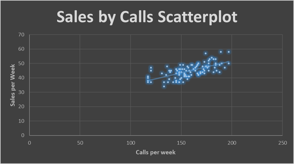
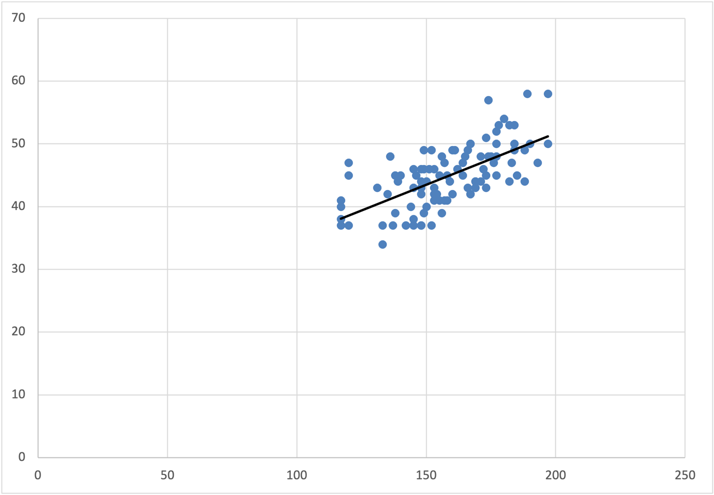
First, the data points were plotted, with the number of calls on the x-axis and sales on the y-axis. Such a manipulation was conducted to identify the relationship between sales per week and calls per week. The scatterplot with a trendline is provided in Figure 1 below. The scatterplot shows a strong positive correlation between calls and sales: sales increase with more calls. The positive correlation was also confirmed by the upward trendline, indicating that an increase in the number of calls led to an increase in sales.
After observing the scatterplot, the correlation was confirmed using statistical tests. In particular, researchers performed Pearson’s correlation and simple linear regression analyses using calls as the independent variable and sales as the dependent variable. Pearson’s r of 0.65 indicated a strong correlation between the variables. Pearson’s correlation coefficient, also known as Pearson’s r, is used to measure the strength and direction of the linear relationship between two continuous variables (McClaive et al., 2018).
Multiple regression analysis, unlike Pearson’s r, is used when it is necessary to quantify the effect of multiple independent variables on a single dependent variable (McClaive et al., 2018). Regression analysis demonstrated that the number of sales can be predicted using the following model:
The regression model had an R² of 0.4228, indicating that changes in the independent variable (Calls) explain 42.28% of the changes in the dependent variable (Sales). Hypothesis testing of the regression model indicated that Calls was a significant predictor of Sales (p < 0.000001). The model suggests that if the number of calls per week increases by one, sales per week increase, on average, by 0.16. This implies that a salesperson needs around 6.25 calls to make one sale. However, the actual average increase in sales will be between 0.113544 and 0.215601 with 99% certainty. All the steps conducted to arrive at the result are provided in Appendix A.
Implications
The implications of the regression model are best described using an example. For instance, let us assume that a salesperson makes 158 calls per week. The regression model implies that one can be 99% confident that the actual average sales per week falls between 43.8 and 45.8 when the number of calls per week equals 158. However, such an estimation does not account for the variability in the number of sales per week.
A 99% confidence interval was calculated for predictions to estimate the range of possible weekly sales observations. The analysis demonstrated that the 99% prediction confidence interval was[34.960211; 54.634965]. This implies that individual future sales predictions, based on 158 calls per week, will fall between 35 and 55 per week. In summary, if sales personnel make 158 calls weekly, this will result in 35 to 55 weekly sales, with an average of 43.8 to 45.8 sales per week.
Limitations
While the regression model discussed above provides accurate estimates, it has limitations. One of the central limitations is the inability to predict sales outside the range of the sample values. This model was created based on a range between 117 and 197 calls per week.
Extrapolations, or predictions outside this range, may be associated with lower accuracy. There are several reasons that extrapolations tend to be less accurate than interpolations. For instance, extrapolation assumes that the relationship between the variables remains the same beyond the observed range.
However, other factors or influences may take effect outside the range. At the same time, the assumption of linearity may be invalid outside the data, leading to inaccurate predictions. This way, the closer the predictions are to the sample’s range, the more accurate they tend to be.
Conclusion
In conclusion, the statistical analysis results indicate a correlation between weekly sales and weekly calls, suggesting that an increase in calls per week is associated with a corresponding increase in sales per week. Therefore, the firm should encourage making more calls to increase sales. In particular, a company can set clear goals for the weekly number of calls and provide training on the role of frequent customer contact.
The introduction of performance-based incentives could also motivate employees. They might be in the form of commission or bonus structures related to the quantity of successful calls or the sales resulting from those calls. Rewards can be monetary, such as gift cards, or non-monetary, like recognition or additional time off. Such interventions can boost the company’s revenues.
Reference
McClaive, J., Benson, G. & Sincich, D. (2018). Statistics for business and economics. Pearson.
Appendix A: Steps
Step 1
Step 2
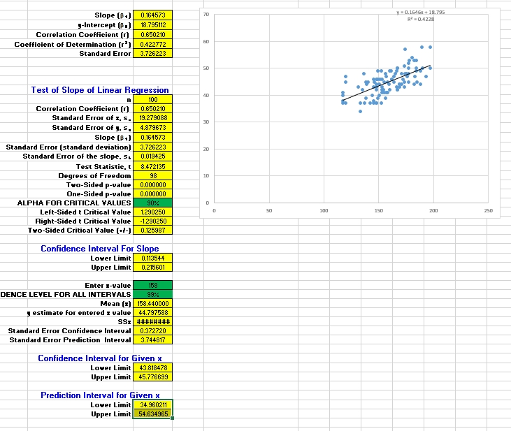
y = 0.1646x + 18.795. Every additional call adds 0.16 sales.
Step 3
r = 0.650210. The coefficient indicates that there is a high degree of correlation between the variables.
Step 4
R² = 0.4228. The coefficient of determination demonstrates that the changes in the independent variable (Calls) can explain 42.28% of the changes in the dependent variable (Sales).
Step 5
Null hypothesis (H₀): β = 0 (There is no relationship between the calls and sales)
Alternative hypothesis (H₁): β ≠ 0 (There is a significant relationship between calls and sales)
Since the significance level is α = 0.10, the critical value is 0.125987. The test statistics was calculated to be t = 8.472135 and the p < 0.000001. Since the test statistics was above the critical value of 0.125987 and the p-value was below the significance level of 0.1, the null hypothesis was rejected, implying that β ≠ 0.
Step 6
The test results suggest that Calls was a significant predictor of sales.
Step 7
95% CI = [0.113544; 0.215601]. The interval demonstrates that the true value of the slope lies between 0.113544 and 0.215601with 99% certainty.
Step 8
Confidence intervals were computed for x = 158. The 99% CI for the dependent variable was [43.818478; 45.776699]. This implies that one can be 99% confident that the true mean value of the dependent variable falls between 43.8 and 45.8 when the independent variable is equal to 158.
Step 9
The 99% prediction CI is [34.960211; 54.634965]. This implies that individual future predictions for sales will be between 35 and 55 for 158 calls per week.
Step 10
Extrapolations appear to be less accurate than interpolation for several reasons. For example, extrapolation suggests that beyond the observed range, the relationship between the variables stays the same. However, there might be other factors or influences that come into play outside the range. Simultaneously, the assumption of linearity may be false outside the data, which implies that the predictions will be inaccurate. Therefore, the predictions tend to be more accurate when they are close to the sample’s range.
Step 11
The results suggest that an increased number of calls is associated with an increased number of sales. Thus, the firm should encourage its employees to make more calls to the customers to increase sales. In particular, a company can establish clear goals and expectations about the number of calls made per week and provide education concerning the importance of making frequent calls to the customer. A company can also offer performance-based incentives to motivate employees. This can include commission or bonus structures tied to the number of successful calls made or the sales generated from those calls. Rewards can be monetary or non-monetary, such as recognition, gift cards, or additional time off.
Appendix B: Excel Output