Introduction
Forecasting future sales with certainty is impossible since the market conditions are unpredictable. The economy is always constantly changing. Despite the uncertainties, management of companies still need to prepare sales forecasts to enable them to prepare a budget for revenue and expenses. The preparation of such budgets is always based on past trends and future objectives of the company. There are serious implications when a company does not achieve its targets. For instance, when the forecasted revenue and net income falls way below forecasted revenue, the share prices of the company are likely to fall. Thus, the management needs to come up with real values when preparing the budgets. This can be achieved by coming up with models that will help estimate the future values of sales revenue. Examples of such models are regression models. The regression models can either be linear or polynomial. Past trends are used to model a regression line. After that, the regression line can be used to estimate future trends. Estimating future values can also be achieved by progressing current values by the proportion of the estimated growth rate of various components of the budgets. The method is commonly used for new business.
Purpose and objectives
This paper aims to carry out an analysis of sales revenue for a company. The analysis will entail coming up with regression models to aid in forecasting the sales revenue of the company for the year 2005 and 2006.
Methods
Historical sales data for the company is provided for five years, that is, between 2000 and 2004. The data is arranged quarterly. The analysis of the data will entail observing the trend of the sales revenue data for the past five years to come with a model that can be used to estimate sales revenue values of the company between 2005 and 2006. There are several methods that can be used to forecast sales revenue. Most methods aim at giving the trend of sales revenue for previous years. After that, a model is estimated to show the relationship between various values. The models generated are tested to ascertain if they are suitable for estimating future values. After that, such models can then be used for future sales revenue. Some of the forecasting models that are commonly used are a linear trend, nonlinear trend and exponential forecasting. Linear forecasting is often preferred since it is timely, accurate, reliable, meaningful, and easy to use. Also, moving averages are often computed to give an overall impression of the pattern of movement of sales revenue over time. Thus they are known as smoothing techniques. In this analysis, regression will be carried to establish a linear relationship between the sales revenue of the company and period time. This linear relationship will be used to forecast sales revenue of the company for the year 2005 and 2006. In addition, graphs and charts will be used to display various trends of the values computed and relationships of various variables. Excel will be used to carry out various computations and analysis.
Analysis
This section comprises of an extensive review of the sales revenue data provided. Some of the areas that will be discussed below are an analysis of the original data, correlation coefficient, linear regression model, variations in the data, analysis of various components of the data, prediction of values, testing the regression model estimated and forecasting the sales for 2005 and 2006. Various statistical tools will be used to reviewing the data provided and coming with a sales forecast.
Analysis of the original data
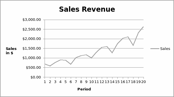
As mentioned above, the sales revenue data is provided for five years, that is between 2000 and 2004. The data are arranged in quarters. The table below shows the historical data of sales revenue for the company for various periods.
The table shows that there has been a general increase in the sales revenue for the company for five years. In the first quarter of 2000, the total amount of sales revenue increased from $684.20. The value increased to $2,639.40 in the last quarter of 2004. It can be observed that the company recorded a decline in sales in the second quarter of all four years. For instance, in 2000, the sales declined from $684.20 in the first quarter to $584.10 in the second quarter. Similarly, in 2001, the sales declined from $885.40 in the first quarter to $677.00 in the second quarter. The same trend was observed in 2002. The number of sales declined from $1,163.10 in the first quarter to $993.20 in the second quarter. Also, in 2003, the number of sales declined from $1,596.20 in the first quarter to $1,260.40 in the second quarter. Finally, in 2004, the number of sales declined from $2,107.80 in the first quarter to $1,650.30 in the second quarter. There was an increase in sales for the third and fourth quarter for all the years. The graph below shows the trend in sales revenue for the 20 periods in the five years.
Correlation coefficient
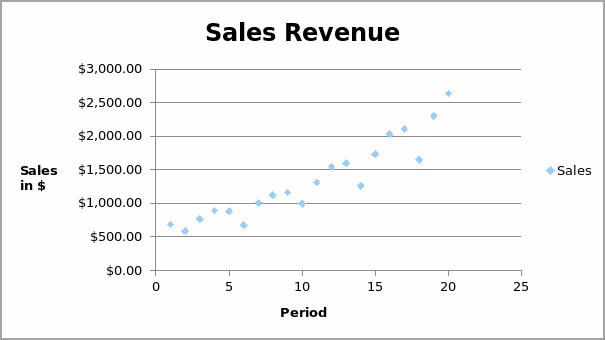
The correlation coefficient measures the degree of relationship between two variables. A positive value of correlation coefficient implies that the variables being investigated have a positive relationship that is, an increase in one value leads to a decline in the other variable. On the other hand, a negative value implies that the variables have a negative relationship. That is, they move in opposite directions. As the value of one variable increases, the value of the other variable declines. A high value of the correlation coefficient shows that the values have a strong relationship. The correlation coefficient between sales revenue and time is 0.9341. This implies that there is a strong positive relationship between sales revenue and time. That is, sales revenue increases over time, as shown in the scatter diagram below.
Linear regression model
Regression analysis is a statistical tool that is used to develop approximate linear relationships among various variables. Regression analysis formulates an association between several variables. There are several variables that can affect the sales revenue of a company. Some of the factors are price charged for the products of the company, competition, news about the company, and the amount spent on advertising, among other factors. When more than one factor is used when coming up with the regression equation, then a multiple regression analysis will be used. However, in this case, a simple regression will be used. When coming up with the simple linear regression model, it is necessary to separate between dependent and independent variables. The dependent variable is the sales revenue, while the independent variable is the period.
The regression line will take the form Y = b0 + b1X
Y = Sales revenue
X = Time
The theoretical expectations are b0 can take any value and b1 > 0 (positive).
Regression Results
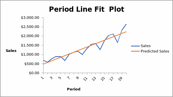
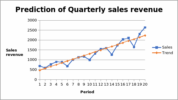
From the above table, the regression equation can be written as Y = 375.1758 + 92.62564X. The intercept value of 375.1758 represents other variables that affect the average sales revenue but are not included in the modelling. The coefficient value of 92.62564 implies that as time increases by one unit, the sales revenue increases by 92.6256 units. When the regression equation is compared with the scatter diagram, there is an indication of consistency. The graph of average sales revenue and time shows an upward trend with a correlation coefficient of 0.9341. The regression equation above also yields a positive slope. Thus, it is clear that the regression equation is sensible. The graph below shows the graph of the original plots of sales revenue and time with a line of best fit.
Variation of the sales data
Measurement of variation of sales revenue data provided is of utmost importance. It shows the extent to which the data for sales revenue will deviate from the average. There are several ways of measuring the extent of variation in the amount of sales revenue. A commonly used method is by computing the variance and standard deviation of a stock. The two approaches measure the volatility of sales revenue. High variance and standard deviation indicate a high variation from the mean value. A low value of variance and the standard deviation is suitable since it shows low variation from the mean. Another tool that is often used to measure variation is the coefficient of variation. It is the ratio of mean and standard deviation. The ratio is regarded as superior since it brings the average of the asset being discussed in context when analyzing the standard deviation of the asset.
The variance, standard deviation and coefficient variation of the sales revenue are quite high. This implies that there is a high variation from the average sales value of $1,347.75. It implies that the sales value can go as low as $761.62 and as high as $1,934.361. The high variations weaken the regression model that will be used for estimating future values. It is because high variation results in a higher value of the residual sum of squares. This creates the need for smoothing the data using moving averages.
Comparisons of yearly sales data
The section will compare the sales data for the four quarters of the five years. The graph below shows the trend of values.
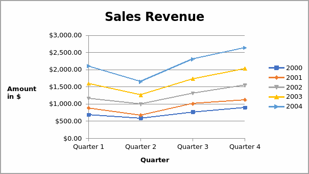
There is an increase in sales revenue over time. The sales data for 2004 are higher than those for the earlier years. From the graph, it is also evident that the sales revenue in all the years increased with a sharp decline in the second quarter. Thus, it is evident that there is a general increase in sales revenue within the quarters of all the years.
Trend and ratios
The trend values are obtained by using the regression line to estimate the value of the sales revenue. Ratios of original and fitted sales revenue data are obtained. The graph of the ratios per quarter is different from the graph of the original sales data per quarter. The gap in years closes in when ratios are used. The values for all the years declined from the first quarter to the second quarter. After that, there is an increase but at a slower rate and the graphs tend to close into a common point.
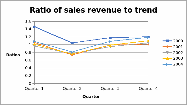
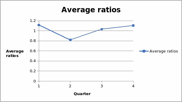
The average ratios above display the general trend of the ratios for each of the years. It displays the same trend as discussed above. They declined from the first quarter to the second quarter and after that an increase. This can be displayed in a graph illustrated below.
Prediction of values
The regression model estimate above, that is, Y = 375.1758 + 92.62564X can be used to predict future values of sales revenue. Such model gives an estimation of the values and not the exact values. However, before the model can be used for prediction, it is necessary to evaluate if it is suitable and can be used for prediction. The two criteria that will be used for prediction are the coefficient of determination and testing the statistical significance of the variable.
Coefficient of determination
Coefficient of determination estimates the number of variations of the dependent variable explained by the independent variables. A high coefficient of determination implies that the explanatory variables adequately explain variations the sales revenue. A low value of the coefficient of determination implies that the explanatory variables do not explain the variations in sales revenue adequately. For this regression, the value of R2 is 87.26%. This implies that time period explains 87.26% of the variation in the price of houses. It is an indication of a strong explanatory variable. Also, the value of adjusted R2 is high at 86.55%. Thus, the regression model is suitable and can be used for prediction.
Testing the statistical significance
Testing statistical significance shows whether the explanatory variable is a significant determinant of the price of houses. A t-test will be used since the sample size is small. A two-tailed t-test is carried out at a 95% level of confidence.
Null hypothesis: Ho: bi = 0
Alternative hypothesis: Ho: bi ≠ 0
The null hypothesis implies that the variables are not significant determinants of demand. The alternative hypothesis implies that variables are a significant determinant of demand. From the table above, the values of t – calculated are greater than the values of t – tabulated. Therefore, the null hypothesis will be rejected, and this implies that the period is a significant determinant of the explanatory variable at the 95% level of significance. The value of the intercept is not relevant when testing the significance of the regression variables. Since the explanatory variable is statistically significant, it implies that the regression line can be used for prediction.
Other tests that can be carried out are tests for multicollinearity, autocorrelation and linearity, among others. From the two tests conducted above, it is evident that the regression model is strong enough and can be used to predict future values of sales revenue. The values predicted will be a continuation of the straight line shown in the graph below.
The graph below shows the trend of trend and ratios that can be used for prediction.
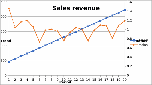
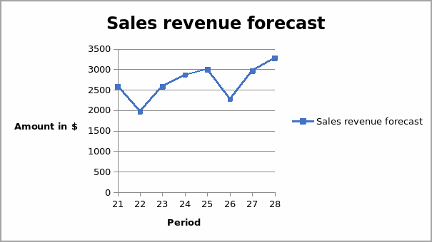
From the above analysis, the regression model can be used for estimation. Thus, the estimated values for sales for the year 2005 and 2006 are shown in the table below.
From the graph above, the forecast shows that there will be an increase in sales for 2005 and 2006. The forecasts for the two years will follow the same trend as the previous years. That is, a decline from quarter one to quarter two and an increase thereafter, as shown in the graph below.
