Section – A. Polymers
Structural factors that promote the crystallization of polymers are the following.
Structural Regularity
A polymer with a regular structure is more likely to crystallize as the ordering of the molecules is easier in that case. A polymer with an irregular structure will not crystallize.
Stereoregularity
This refers to configurational and structural isomers of the monomers being arranged in the polymer chain. The presence of such isomeric regularity in a polymer promotes the crystallization of a polymer.
Skeletal Regularity
Linear polymers are easier to crystallize. The difficulty for crystallization increases with branched polymers and further for network polymers.
Tacticity
This refers to the repeat units being configurational isomers. In this case, crystallization is easier.
Geometric Isomerism
This refers to the repeat units being geometric isomers. In this case, crystallization is easier.
Structural factors that control the melting temperature of crystalline polymers are the following.
The extent of cross-linking
If the extent of cross-linking is more than the melting temperature of the crystalline polymer will be higher. This is because more energy is required to break the cross-links in the polymer.
Presence of bulky side groups
The presence of bulky side groups increases the melting temperature of crystalline polymers.
Attractive intermolecular interaction
The presence of attractive intermolecular forces means higher energy will be required to break this force of attraction. Therefore, the melting temperature of the crystalline polymer will be high.
The high density of hydrogen bonds
A certain amount of energy (25 kJ/mol) is required to break hydrogen bonds. Therefore, the higher is the density of hydrogen bonds in a crystalline polymer, the higher will be its melting point.
Chemical structure of the given polymers are the following.
- CH3COCH3 and CH3COOH
- C6H5COOH and C2H5COOH
Polymerization process for the given polymers is listed below.
- Chain polymerization
- Step polymerization
Bragg’s law of diffraction relates inter-planer spacing of a crystalline solid with the angle of diffraction produced by X-rays of a certain wavelength. Bragg’s law for diffraction is stated below.
“Twice the product of inter planer spacing dhkl of the certain plane (h, k, l) of a crystalline solid and sine of the angle for corresponding diffraction peak equals an integral multiple of the wavelength of the X-ray used to produce the diffraction pattern”.
Mathematically, this law can be stated as
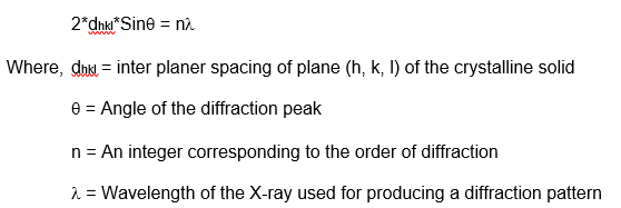
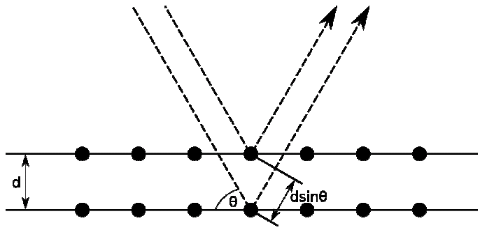
As shown in the figure below, when X-rays are made to an incident on a crystalline material, they reflect from successive planes. The inter planer spacing of the crystalline material produces a path difference between the X-rays reflected from successive planes. The magnitude of the path difference caused by two successive planes with spacing ‘d’ is 2dSin. Only when this path length equals an integral multiple of the wavelength , the peaks of the Electromagnetic fields will coincide and constructive interference will be possible leading to a diffraction peak. A is fixed and for a plane ‘d’ is also fixed, the diffraction peak can be detected by scanning the detector over i.e. the diffraction angle.
Difference between the standard engineering definition of stress and strain and that for true stress and strain is explained below.
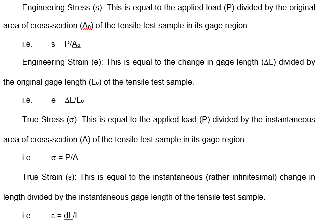
Under inhomogeneous deformation conditions or necking, it is good practice to use the latter definitions to take into account the impact of strain hardening without shadowing it due to geometrical softening (due to reduction in the cross-section caused by necking).
Fracture toughness of a material is a quantitative measure of the resistance offered by the material to the crack propagation through it. This is defined as (1)

Here, KIC = Fracture toughness of the material
- σ = Nominal Applies Stress
- ac = critical crack length beyond which catastrophic fracture occurs
In the case of ductile material, a plastically deformed zone is always presented ahead of the crack tip. The formation of a plastic zone ahead of the crack tip consumes a significant amount of energy and therefore, the material is tougher. This is not so in the case of brittle ceramics, which cannot deform plastically due to the presence of directional electrostatic or covalent bonding, while ductile materials can easily deform due to the presence of directionless metallic bonding. This is the reason, why ductile materials are tougher than ceramics.
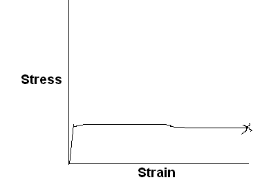
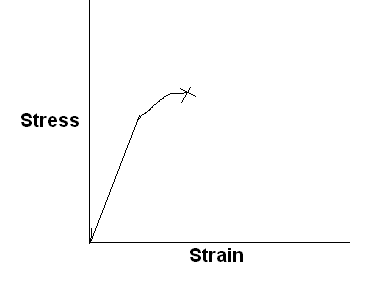
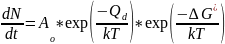
Characteristic stress-strain curve for a different kind of polymeric material is sketched below, with labels showing significant features of the curve.
Stiff, strong, and brittle polymer
Stiff, strong, and tough polymer
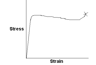
Ductile polymer
Lightly cross-linked elastomeric polymer
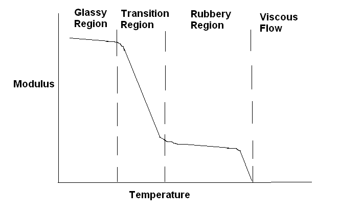
Following diagram shows the variation in the modulus of a polymer (undergoing a transition) with temperature. Different regions of this process are also shown in this diagram.
Two kinetic processes that generally control the rate of phase nucleation and growth are the following.
- Formation of the interface between the existing phase and new phase by Energy fluctuation of the size ΔG*
- Frequency of with which atoms from liquid attach to solid νd or rate of diffusion of solute through the existing phase
Variation in the individual rates of these kinetic processes with temperature is shown in the following figure.
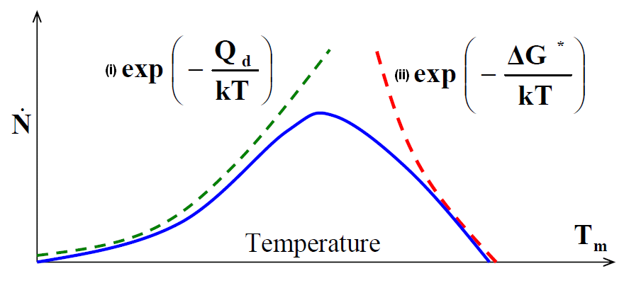
At a given temperature below Tm, the size of ΔG* will decrease, while the value of Qd (Diffusion coefficient) will remain the same.
Therefore, there is an optimum temperature below Tm or an optimum undercooling (ΔT) at which the rate of phase transformation is maximum.
Section – B
A typical tensile stress-strain curve for a brittle ceramic and a ductile metal alloy is sketched below.
Referring to the figure below, which is a typical stress-strain curve of a ductile material the main material parameters that can be measured from a tensile test are briefly defined below.
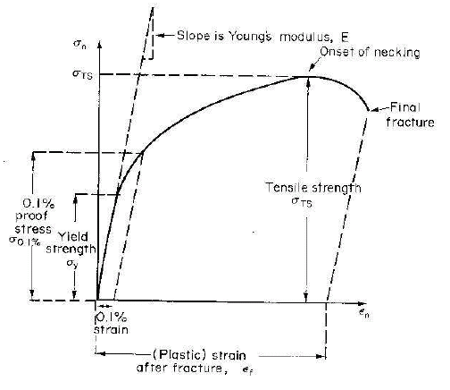
Elastic Modulus
This is the slope of the curve in the elastic or linear region of the stress-strain curve.
Yield Strength
This is the stress at which yielding or plastic deformation of the material begins in the tensile test. In case this point is not distinct, proof stress corresponding to 0.2% (or a suitable value) plastic strain is chosen. A line from 0.2% plastic strain is drawn parallel to the linear or elastic region of the curve is drawn and the stress value where it cuts the stress-strain curve is taken as the yield strength of the material.
Ultimate Tensile Strength
This is the maximum stress in the tensile stress-strain curve.
% Elongation
This is a measure of the ductility of the material. This is the maximum plastic strain the material can withstand before fracture.
Uniform Ductility
This is the plastic strain until the onset of necking and this is a very important parameter for a material. If this value is large, the material possesses good formability.
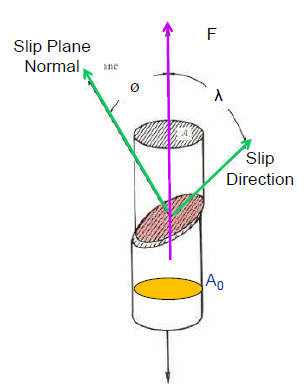
When a ductile metal reaches its yield strength, dislocations start moving within the grains and contribute towards plastic or permanent deformation of the material. At yield stress, the resolved shear stress on a slip plane in a crystal increases the critical resolved shear stress (CRSS) for that material as shown in the figure, below.
Four mechanisms by which yield strength of a ductile alloy can be improved are the following.
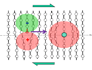
Solid solution hardening
When a solute of a different size than the solvent atoms is put into the lattice, it causes lattice distortion. This lattice distortion interacts with the strain field around the moving dislocation and hinders its motion, thereby causing the strengthening of the alloy as shown in the following figure.
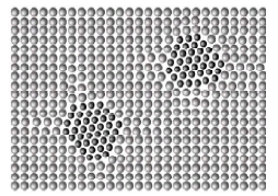
Precipitation Hardening
Small and coherent precipitates (figure below) in a matrix lead to the strengthening of the alloy. This is because the moving dislocation will have to either cut through these precipitates or loop around them. In both cases, the length of the dislocation increases, and more energy/force is required for the motion of dislocations, and thus the strength of the alloy increases. This was discovered in the aluminum-copper system and widely used for a variety of aluminum alloys.
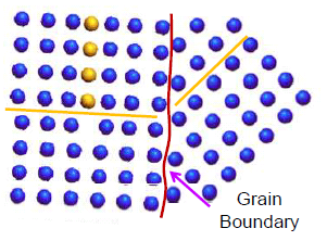
Grain refining
Grain boundaries are an effective barrier to dislocation movements. Therefore, grain refining will lead to finer grains i.e. more grain boundaries and more barriers for dislocation movement. Thus grain refining leads to the strengthening of a ductile alloy.
Strengthening due to grain refining is given by the famous Hall-Petch relationship which states that strengthening due to grain refining is inversely proportional to the square root of grain size.
Strain Hardening
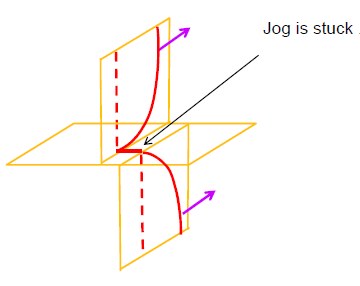
If the material is deformed plastically, it leads to the generation of more and more dislocations in the material. These dislocations interact with each – other and impede the motion of each – other; thus producing strengthening of the material. Many times interaction of these dislocations leads to formations of immobile Jogs (Figure below) and these immobile jogs contribute significantly to the strengthening of the material. This is produced by the cold working of the material.
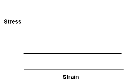
Stress-strain curve for an ideally elastic solid and a viscous liquid are sketched below.
An ideally elastic solid

A viscous liquid
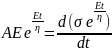
A spring and a dashpot can be combined in series (figure below) to form a Maxwell unit.
The spring has an elastic modulus of E and the dashpot has a viscosity of η.
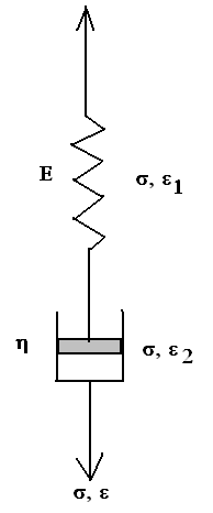
This combination of the spring and the dashpot is loaded to the overall stress of σ. As the two are in series, therefore, the stress in the individual components (spring and the dashpot) will be the same and equal to the overall stress σ. The strain, however, will be different.
Let us assume strain ε1 in the spring and ε2 in the dashpot.
 &
& 

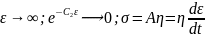
Because, the Spring and the Dashpot are in series, therefore,
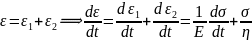


Multiplication by a factor eEt/n for integration leads to
 ; where, C is the constant of integration At t = 0, σ = 0; thus, C = Aη
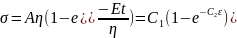

 i.e. for large strains, the Maxwell unit will behave like flow in the Dashpot or viscous liquid.
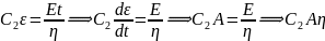
Given, C1 = 3*1010 N/m-2 and C2 = 2
Therefore, the modulus of this polymer will be
E = C1*C2 = 6*1010 Pa = 60 GPa
Molecular masses of three polystyrene samples are given below.
- Sample 1: Molecular mass = 10,000 g/mol
- Sample 2: Molecular mass = 40,000 g/mol
- Sample 3: Molecular mass = 90,000 g/mol
Number average molar mass will be calculated by taking an equal number of moles (for example 1 mole of each sample) and dividing the total mass by the sum of the total number (here 3) of moles.
Number Average Molecular Mass = (10,000 + 40,000 + 90,000)g/(1+1+1) mol = 46667 g/mol.
Weight average molar mass will be calculated by taking the equal weight from each sample. This means, if we take one mole of sample 3, then one needs to take 2.25 moles of sample 2 and 9 moles of sample 1. Then the total mass of polystyrene thus taken together will have to be divided by the total number of moles.
Therefore, Weight Average Molecular Mass = (10,000*9+40,000*2.25 + 90,000*1)g/(9+2.25+1) mol = 22041 g/mol
Principal requirements for the formation of network polymers by step polymerization and significance of gel point in such polymerization are outlined below.
For step polymerization to happen, the chemical reaction between the monomers should be very clean. Further, it should be possible to take chemical reactions to a very high degree of functional group conversion. The stoichiometric ratio of the monomers should be perfect. This calls for very high purity of the monomers. Even with all this suitable strategy needs to be employed to achieve a high degree of cross-linking or molecular weight.
Gel point is the point at which a cross-linked 3D structure is formed. It can form at even low conversion. However, this is not desired at the gel point corresponds to an abrupt increase in the viscosity of the reaction mixture and thus retards further reactions. Therefore, the gel point should not be formed early for a good step polymerization reaction.
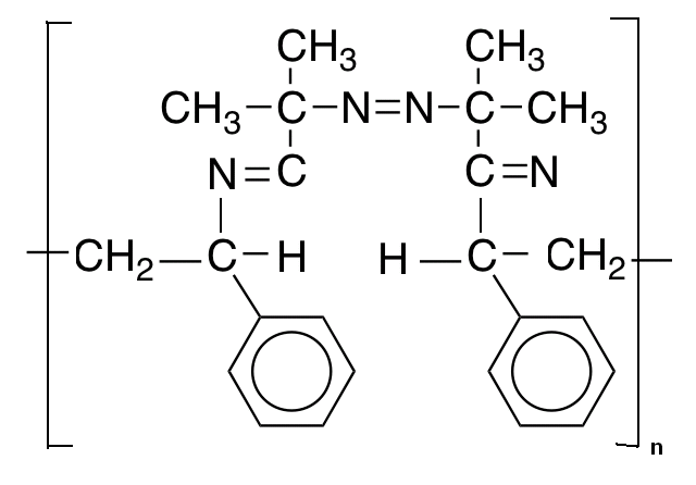
Structure of the polymer formed and type of polymerization for the following polymerization reaction is given below.
- C2H5—O[—(CH2)4—]n—
This is chain anionic chain opening polymerization. This is living polymerization with no formal end. The termination is caused by acidification with dilute sulphuric acid with –OH being the end group.
- –[CO —NH—(CH2)6—NH—CO—O—(CH2)6—O]n—
This is step polymerization.
X-rays are produced by accelerating electrons hitting at the target anode. As the electrons are decelerated in the electric field of electrons in the target, continuous X-rays are produced by Bremsstrahlung. Thus the production of continuous X-rays is guaranteed in any endeavor to produce X-rays. Only if the electrons have sufficient energy to dislodge some of the electrons from the inner or core-shell of the target atom, characteristic X-rays can be produced by electronic transition within the target atom. Thus it is obvious why both continuous as well as characteristic X-rays are generated.
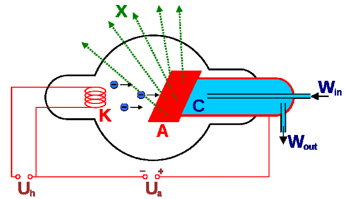
Schematic diagram of Coolidge Tube for X-ray generation
For the production of Kα X-rays, one needs to dislodge electrons from the K-shell of the target atom. Once electrons are dislodged from the K-shell electrons from higher shells will fall into it. Electrons from L-shell will give Kα X-rays, but there is nothing to stop electrons from M-shell to fall into vacant K-shell and that will lead to the generation of Kβ X-rays. Thus the generation of Kα X-rays is not possible without also producing Kβ X-rays.
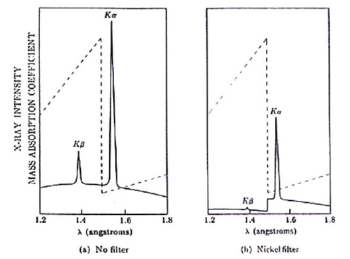
Cu Kα and Kβ radiations are the following:
- Cu Kα = 1.5405 Ao
- Kβ = 1.39217 Ao
K-absorption edge of Zn filter is Kedge (Zn) = 1.2837 Ao
Therefore, the Zn filter will not be able to separate Cu Kα and Kβ radiations. To separate these two X-rays one needs a filter with an absorption edge between the energy of the Cu Kα and Kβ X-rays.
Nickel filter with K absorption edge of 1.4869 Ao is suitable for this task and spectrum of Cu with and without Ni filter is shown below.
X-ray powder diffractometer is also known as the Debye-Scherrer camera. In this camera, the powder sample is loaded in the center of the camera, and the film is wrapped on the wall of the camera (figure, below).
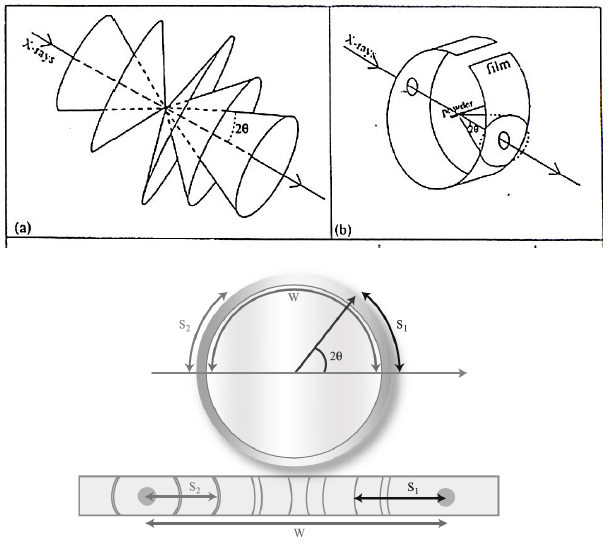
X-rays enter the camera through the hole in the film, strike the powder sample, and get diffracted. The diffraction cone cuts through the film leaving diffraction lines. Angle of diffraction can then be calculated from the distance of the diffraction lines from the center of the hole and the radius of the camera. This angle of diffraction and the wavelength of the X-ray is then used to calculate the d-values using Bragg’s equation.
The values of the d-spacing for the different planes are then converted into integers by multiplying them with suitable constants. The index of the plane is then calculated by using arithmetic and also taking into account extinction planes.
Phase diagram of a binary alloy Ag-Cu, which has a eutectic at 779 oC and Ag-40at%Cu is sketched below. All the relevant phase fields are marked and two tie lines are also drawn for Ag-20at%Cu alloy.
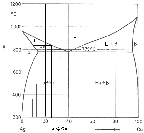
Let us consider the solidification of Ag-20at%Cu alloy. The melt will solidify over a temperature range of ~875 oC to 779 oC. Let us consider a tie line at 850 oC. The melt which will solidify at this temperature will lead to the formation of α and its composition will be Ag-9at%Cu much different from the original Ag-20at%Cu. Further the Cu will be rejected into the remaining melt and the composition of the remaining melt will be Ag-25at%Cu.
This will solidify now and let us consider a tie line for this remaining melt at 800 oC. The solid forming at this temperature will be Ag-13at%Cu and the remaining melt will be Ag-35% Cu. Thus it can be seen from the phase diagram that for solidification of an alloy with Ag-20at%Cu one gets compositional variation (also known as coring as the core is lean in solute and outer is rich in solute) during solidification from Ag-7at%Cu (in the initial solids or core of the primary dendrites) to Ag-40%Cu in the interdendritic eutectic mix.
The microstructure of Ag-20at%cu alloy showing primary dendrites and the interdendritic eutectic mixture is presented below.
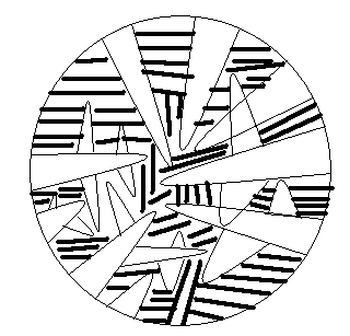
Even though Ag-20at%Cu is well below eutectic composition, during solidification of this alloy, there will be solute rejection into the melt leading to enrichment of the remaining melt by the solute. Finally, there will be a small fraction of melt with eutectic composition and it will decompose into eutectic solid in the interdendritic region as discussed in Q1. (b).