Exploratory Data Analysis
A high school teacher is interested in determining whether his students’ test scores increase over the course of a 12 Week period. Descriptive statistics for students’ test scores for the 12 Week period are provided in Table 1. Of the 12 students who participated in this study, the mean pretest score was 29.58 with a standard deviation of 12.22, the mean for Week 2, Week 4, Week 6, Week 8, Week 10 and Week 12 scores with standard deviations were: 33.08, SD = 10.11; 35.42, SD = 9.89; 35.67, SD = 10.67; 39.92, SD = 9.72; 45.67, SD = 8.69 and 50.00, SD =10.19 respectively. The minimum pretest score was 16 and the maximum score was 59 whereas the minimum Week 2 score was 22 and the maximum was 60.
During Week 4, the minimum score increased to 27 whereas the maximum score increased to 63. The minimum and maximum scores for Week 6 were 20 and 60 respectively (indicating a slight decrease in the maximum score) while the minimum and maximum scores for Week 8 were 28 and 65 respectively. During Week 10, the minimum score increased to 33 whereas the maximum score increased to 67. Finally, in Week 12, the minimum test score reached the highest score in the entire course period (34) which was similar to the maximum score (73). All the skewness and kurtosis values for the scores in the entire course period were positive indicating that the scores were symmetrical.
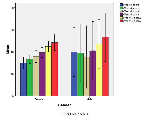
Figure 1 gives a visual display of test scores over the 12 weeks course according to gender. The clustered bar charts with error bars clearly indicate that the mean test scores for females had an increasing trend throughout the course. However, test scores for males were high in Week 2, declined slightly in Week 4 and Week 6 and then increased consecutively up to the end of the course (Week 12). It is also evident that in general, males had higher mean scores in all the test periods except in Week 6 where the mean scores for females were slightly higher. These findings were confirmed in Table 2 which displays mean test scores for males and females over the 12-weeks long course.
Table 2 clearly indicates that the mean pretest score for males (32.25, SD =19.43) was higher than that of females (28.27, SD = 8.17). Week 2 mean score was also higher for males (39.75, SD = 13.89) compared to the mean score for females (29.75, SD = 6.32). This was the same trend in Week 4, males (39.00, SD = 16.43) against females (33.62, SD = 5.18). It is notable that the mean for males reduced slightly compared to Week 2 scores. During Week 6, the mean score for males dropped (35.25, SD = 17.80) and females had a slightly higher mean score (35.88, SD = 6.56).
The mean test scores for males however increased and exceeded those of females during Week 8, males (41.00, SD = 16.63) against females (39.38, SD = 5.37). The mean test scores for males in Week 10 (47.25, SD = 13.96) was still higher compared to that of females (44.88, SD = 5.74) and this trend was maintained in Week 12 test, males (53.25, SD = 10.19) versus female’s (48.38, SD = 8.52).
Repeated Measures ANOVA
Repeated-measures ANOVA was conducted to determine whether student’s scores increased over a 12 weeks course. The Wilk’s lambda for scores is significant, F = 20.44, p =.002 and this is greater than.05 but this it is not significant, F =.80, p =.607 for scores*gender (Table 3). All the other F values in Table 3 are signs indicating that the assumption of sphericity has been violated. Table 6 shows that there is no interaction between scores*gender, F(1, 25.54) =.40, p>.05 since the F critical value is greater than.05 (p =.539). This implies that gender and different time periods when tests are taken do not combine to affect the test scores attained by students.
The lower bound for epsilon as per Table 4 is.167 and this is the lowest value the epsilon can be. Sphericity for this data has been violated since Mauchly’s W is significant, W(20, 56.88) =.001, p =.001 (this is less than.05) as shown in Table 4. This indicates that the variances differences between the differences of scores in different time periods are unequally calling for adjustment using the Greenhouse-Geisser epsilon or a multivariate test. In this case, the Greenhouse-Geisser epsilon was used.
From the sphericity assumed row in Table 5 sphericity F(6, 3246.54) = 20.61, p<.001 has been violated. This has been corrected using the Greenhouse-Geisser epsilon but the F value still remains significant F(2.65, 3246.54) = 20.61, p<.05 hence sphericity is still violated and the critical values F are not valid. It is however notable that in the Scores*Gender test, the F value is significant, F(2.65, 3246.54) = 20.61, p=.341 (greater than.05) after Greenhouse-Geisser epsilon adjustment. The F value is therefore valid and the variances differences between the differences of gender and times scores are assumed to be equal.
There is no main effect of gender, F( 1, 290.72) =.480, p>.05 as indicated in Table 7 since the F value for gender is not significant (p =.504 and this greater than.05). This indicates that the gender of the student does not act significantly to determine the scores attained by students at any time of the test during the 12-week course. There was no need for post-hoc tests since gender has less than three groups yet post hoc tests are performed if the a variable has at least three groups.
There is a main effect of time of test scores, F(1, 2962.68) = 46.91, p<.05 as indicated by a significant F value of p =.001 (Table 6). This implies that there is a change (increase) of scores from Week 0 to Week 12. To understand at what times scores increased or decreased in the course period, a post hoc test (LSD) was conducted.
After conducting LSD post hoc test (Table 8), it was evident that there was no significant increase in test score, p =.213 from Week 0 to Week 2 (91 CI range from -12.04 to 3.04). However, there was a significant increase in test score, p =.031 from Week 0 to Week 4 as was the case in Week 0 to Week 6, p =.031. A comparison between Week 0 and Week 8 shows that there was a significant increase in test scores, p =.004 and this was also observed in Week 10, p =.001. From Week 0 to the end of the course (Week 12), there was a significant increase in test score, p =.001. Comparing Week 2 to Week 4, there was no significant increase in test score (p =.335 and this is greater than.05).
In the same way, there was no significant increase in test score from Week 2 to Week 6, p =.734 but there was a significant increase in test score when comparing Week 2 with Week 8, p =.018. Comparing Week 4 with Week 6, there was a significant increase in test score, p =.510 but there was a significant increase in test score when comparing Week 4 with Week 8 scores, p =.004. Comparing Week 6 to Week 8 scores, there was a significant increase in test scores, p =.001. From Week 8 to Week 12, the test scores increased significantly, p <.05. The findings in Table 8 therefore indicate that there was an overall increase in test score with time except in a few cases as explained by the post-hoc analysis.
Applying Analytical Strategies to an Area of Research Interest
I have an interest in working as an International Police Advisor (IPA) for the benefit of our Homeland Security. As an International Police Advisor, there are several responsibilities that I will be required to handle. Partnering with the U.S. military personnel to provide skilled persons in civilian law enforcement will be one of the main responsibilities. International Police Advisors can serve in Border and Point of Entry in order to enhance law at the borders and particularly prevent entry of illegal persons, drugs, and weapons among other crimes. A great concern to the United States Homeland Security has been the identification of persons who are likely to engage in acts of terrorism or general crime.
Positive identification of likely criminals requires a thorough understanding of human behavior. In specific, an understanding of past criminal activities can be used to predict the likelihood of engaging in unlawful practices. In relation to my area of interest as an IPA, I would suggest conducting research to identify whether there is any relationship between prior engagement in misconduct, past experiences and delinquency and the likelihood of engaging in serious criminal activities.
This can form a concrete and dependable ground for criminal investigations. In this study, it would be advisable to examine individual’s prior marriage relationships in order to predict involvement in crime. This is based on Sampson and Laub (1993) argument that if persons who are in the verge of entering adulthood get involved in marriage relationships, their likelihood in engaging in crime is significantly reduced. As such, persons with unstable or no marriage relationships in the transitory period are more likely to engage in criminal activities.
Xu (2006) observes that there is tendency of having persistent antisocial behaviors in the entire life of a person. In that case, it is possible to study the existence of juvenile delinquency as a predictor of adulthood delinquency. On the same aspect, identifying various social factors such as social networks as well as social capital would help predict involvement in criminal behaviors. In addition, this study would look into whether gender influences involvement in antisocial activities. From the understanding of the above questions, it would be possible to prevent criminals from perpetrating their heinous acts thus proving beneficial to the Department of Homeland Security.
According to Leech, Barrett and Morgan (2005), repeated measures ANOVA is most suitable when there is a single independent variable which has at least two levels that are repeated measures and a single dependent variable. Also notable is that repeated measures ANOVA is carried out when “the same measurement is made several times on each subject or the same measurement is made on several related subjects” (Leech, Barrett and Morgan 2005, p. 163). In this case, gender of the participant would be an independent nominal variable (0 = Female, 1 = Male). On the other handle, number of criminal records is the dependent variable and this would be scale data.
The number of criminal records would be determined for the participants (males and females) during the age of 15 years, 20 years, 25, 30 years, years, 35 years and 40 years indicating that there would be six levels of measurement. Gender would be a fixed factor whereas number of criminal records would be a repeating factor measured during the six time periods. Using these variables, it would be possible to determine whether there exists a main effect of gender on delinquency and the main effect of different ages on delinquency.
To identify whether the assumption of sphericity is violated in the data, one is supposed to look at the Mauchly’s Test of Sphericity output. If the Mauchly’s W value is significant (p<.05), this indicates that sphericity is violated, otherwise the assumption of sphericity holds. If the assumption of sphericity is violated, it implies that the critical F values are invalid (the variances of differences between the variables are unequal) and this would require correction. Correction of the F-value is made by adjusting the degrees of freedom for the F-value with a factor that is generated as the Greenhouse-Geisser epsilon or Huynh and Feldt epsilon (Field, 2009).
References
Field, A. (2009) Discovering statistics using SPSS (3rd Ed.). Los Angeles: Sage. Web.
Leech, N. L., Barrett, K. C. and Morgan, G. A. (2005). SPSS for intermediate statistics: use and interpretation (2nd Ed.). New Jersey, NJ: Lawrence Erlbaum Associates, Inc., Publishers. Web.
Sampson, R. J., and Laub, J. H. (1993). Crime in the making: pathways and turning points through life. Cambridge, MA: Harvard University Press.
Xu, Q. (2006). From juvenile delinquency to adult criminal behavior: expanding the state dependence perspective on persistent criminal behavior. Not Published. Web.
Appendix
Table 1: Descriptive Statistics for Student’s Test Scores over a 12 Week Period.
Table 2: Descriptive Statistics for Test Scores according to Gender during the 12 Weeks Course.
Table 3: Multivariate Tests for Test Scores and Gender.
Table 4: Mauchly’s Test of Sphericity for Test Score Data.
Table 5: Tests of Within-Subjects Effects of Scores and Scores*Gender Interaction.
Table 6: Tests of Within Subjects Contrasts for Scores and Scores*Gender.
Table 7: Tests of Between-Subjects Effects Significance Table.
Table 8: Post-hoc Test to Explain the Main Effect of Time.