Introduction
The current paper provides the results of two multiple regressions performed on the same data but using different types of coding of dummy variables: dummy coding and orthogonal coding. After the description of the data file and after testing the regressions’ assumptions, the research questions, hypotheses, and the alpha level are specified; next, the results of the statistical tests are supplied. The paper is concluded with an analysis of the strengths and limitations of the two types of coding of dummy variables.
Data File Description
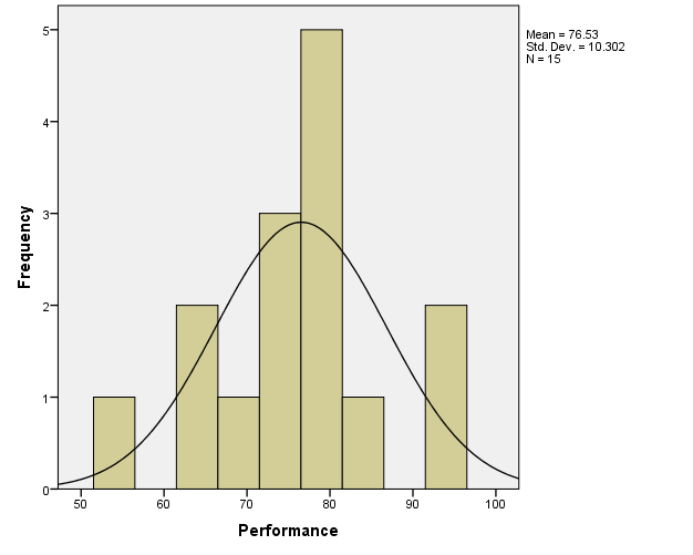
The data set contains results of a survey aimed at assessing the impact of anxiety on exam performance. The outcome variable is Performance, which is measured on an interval/ratio scale. The ordinal predictor variable, Anxiety, was dummy coded using dichotomous variables D1 and D2, and orthogonally coded using nominal variables O1 and O2. The sample size is N=15.
Testing Assumptions
From the histogram provided in Figure 1 below, it is apparent that the normality assumption is not significantly violated for the Performance variable.
Research Question, Hypothesis, and Alpha Level
For the dummy-coded regression, the research question is: “Do levels of anxiety predict exam performance?” The null hypothesis for the overall regression is that the levels of anxiety do not predict exam performance (i.e., the means of performance do not differ significantly). The alternative hypothesis is that the levels of anxiety predict exam performance (i.e., at least two means differ significantly). For D1, the null hypothesis is that there is no significant difference in exam performance between the medium- and low-anxiety groups; the alternative hypothesis is that there is such a difference. For D2, the null hypothesis is that there is no significant difference in exam performance between the medium- and high-anxiety groups; the alternative hypothesis is that there is such a difference. For the orthogonal-coded regression, the research question, and the null and alternative hypothesis for the overall regression are the same as those for the dummy-coded regression. However, for O1, the null hypothesis is that there is no significant difference in exam performance between the high- and low-anxiety groups; the alternative hypothesis is that there is such a difference. For O2, the null hypothesis is that there is no significant difference in exam performance between the mean of the medium-anxiety group and the combined means of the low-anxiety and high-anxiety groups; the alternative hypothesis is that there is such a difference. Because no rationale is provided for choosing the α-level, the standard α=.05 will be used for the tests.
Interpretation
As was stated before, the Performance variable was judged to be approximately normal, so no transformations were needed.
For the dummy-coded regression, D1=1 for the low-anxiety group, and D1=0 for other groups.
For the orthogonal-coded regression, the dummy variables were coded as shown in Table 1 below:
Table 1. Orthogonal coding of dummy variables for the orthogonal-coded regression.
Both regressions were conducted using the method of forced entry (“Enter”) (Field, 2013).
Dummy-Coded Regression Results
Table 2. Model summary output for the dummy-coded regression.
Table 2 above supplies the model summary. The multiple correlation coefficient R=.738, which indicates a good model fit. The R2=.544, meaning that the model can explain approximately 54.4% of the variance in the data.
Table 3. The SPSS ANOVA output for the dummy-coded regression.
Table 3 above provides the ANOVA output for the regression. In this case, F(2)=7.164, and it is statistically significant at p=.009. Therefore, the null hypothesis for the overall dummy-coded regression can be rejected at α=.05.
Table 4. The SPSS Coefficients output for the dummy-coded regression.
Table 4 above demonstrates the Coefficients output. The b values mean that the performance can be predicted from the regression model as follows (Warner, 2013):
Performance = bConstant + bLowAnxietyGroup*D1 + bHighAnxietyGroup*D2.
The bLowAnxietyGroup and bHighAnxietyGroup coefficients refer to mean differences between the respective group and the medium anxiety group; the latter means is represented by constant.
Both b values were statistically significant:
- bLowAnxietyGroup = -17.600, t(11)=-3.704, p=.003; therefore, the null hypothesis for D1 was rejected, and evidence was found to support the alternative hypothesis. The effect size as measured by squared semi partial correlation was srD1=.52 (large).
- bHighAnxietyGroup = -12.000, t(11)=-2.526, p=.027. Thus, the null hypothesis for D2 was rejected, and evidence was found to support the alternative hypothesis. The effect size as measured by squared semi partial correlation was srD2=.24 (medium).
Orthogonal-Coded Regression Results
Table 5. Model summary output for the orthogonal-coded regression.
Table 5 above provides the model summary. The multiple correlation coefficient R=.738, (a good model fit). The R2=.544, so the model can explain nearly 54.4% of the variance in the data.
Table 6. The SPSS ANOVA output for the orthogonal-coded regression.
Table 6 above provides the ANOVA output for the regression. Here, F(2)=7.164; it is significant, p=.009. Thus, the null hypothesis for the overall orthogonal-coded regression can be rejected at α=.05.
Table 7. The SPSS Coefficients output for the orthogonal-coded regression.
Table 7 above supplies the Coefficients output. constant is the grand mean of Performance, whereas b-values reflect contrasts (Warner, 2013):
- bOrthogonalPositiveLinearTrend = 2.800; it represents the contrast between the low- and high-anxiety groups. Here, t(11)=1.179, p=.261. Therefore, the null hypothesis for O1 was not rejected; the difference between the mentioned groups was non-significant. The effect size as measured by squared semi partial correlation was srO1=.0529 (small).
- bOrthogonalCurvilinearTrend = -4.933; it represents the difference between the mean of the medium-anxiety group and the combined means of low- and high-anxiety groups. In this case, t(11)=-3.597, p=.004; thus, the null hypothesis for O2 was rejected, and evidence was found to support the alternative hypothesis. The effect size as measured by squared semi partial correlation was srO2=.491 (large).
Conclusion
Therefore, both the dummy-coded multiple regression and the orthogonal-coded multiple regression provided the same answers to the overall research question of the analysis (the results were significant). The ANOVA outputs (Tables 2 and 5), as well as the Model Summary outputs (Tables 3 and 6), were equivalent in the two regressions, which indicates that both regressions tested the same overall hypotheses. However, the Coefficients outputs (Tables 4 and 7) were different, which is caused by the fact that the variables are coded differently, and the regressions tested different null hypotheses for the dummy variables.
A strength of the dummy coding is that it allows for directly comparing the groups to one another; for instance, in the current regression, the medium-anxiety group was directly compared to the low-anxiety group and to the high-anxiety group. In addition, the dummy coding allows for easily obtaining the group means for the dependent variable. However, a limitation is that it might be difficult to contrast a number of groups with the same coding. An advantage of orthogonal coding is that it permits for more easily contrasting different groups to one another, or for comparing one group to the rest of the groups. A disadvantage, however, is that is somewhat more difficult to calculate the group means for the dependent variables.
References
Field, A. (2013). Discovering statistics using IBM SPSS Statistics (4th ed.). Thousand Oaks, CA: SAGE Publications.
Warner, R. M. (2013). Applied statistics: From bivariate through multivariate techniques (2nd ed.). Thousand Oaks, CA: SAGE Publications.