Tarot LTD: Work in a Competitive Market

Tarroc LTD

Points to note:

• Tarroc is making normal profits.
• The industry is at its ‘long-run’ equilibrium.

The scenario is given of the industry in which Tarrot LTD operates implies a purely competitive market. It is characterized by a large number of relatively small firms. These firms are considered price takers being that no single firm can influence the market price.

The following diagram attempts to show the demand for and supply of carrots (as the output) and the long-run equilibrium Tarroc LTD.

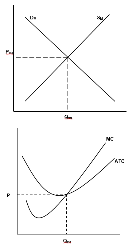
S_M and D_M are a representation of the market supply and market demand functions, respectively. Since we are in a scenario whereby the market is in equilibrium, the equilibrium quantities and price are Q_eq and P_eq respectively. It should however be noted that the quantities measured along the Q-axis in the diagram for the industry represent large quantities while those measured along the Q-axis in the diagram for the firm are relatively small. This is because the firm accounts for a very small share of goods offered for sale in the market. After all, in this industry, there is a large number of small producers.

Given that the major health benefit linked to the consumption of carrots has received widespread publicity, our economic sense would tell us that the demand for this product will increase. The following diagram attempts to illustrate the short-run effects of this change in demand on market equilibrium and on Tarroc’s production.

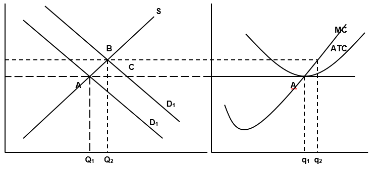
The outcome of an increase in demand is a greater quantity demanded at a given price level. This is a typical example of a demand shift. An increase in demand from D to D₁ moves the short-term market equilibrium from point A to B. The output rises to point Q₂ and consequently the price increases to P₂. The price increase corresponds to the rise of the demand curve of Tarroc LTD from D to D₁ in the firm’s diagram. Tarroc LTD responds to the higher price by increasing its output to Q₂ and is seen to earn economic profit as illustrated. This implies that, for a single firm (in this case Tarroc), the increase in price raises marginal revenue from MR₁ to MR₂. That is why Tarroc responds in the short-run by increasing its output to Q₂.

Given a scenario where the effects of the shock in (b) above are permanent (and hence go into the long-run), the market will adjust in the following ways in the long-run:

A mechanism commonly known as the Long-run Adjustment Process will be used. This mechanism implies that the short-run ‘super-normal’ profits of a firm under perfect competition (in this case, Tarroc LTD), gets transformed to normal profits in the long run. It also suggests that in the long-run, no firm will continue to produce even at the least loss. This is to say that, after the long-run adjustments have come to completion (i.e. when long-run equilibrium is achieved), the price of carrots will be exactly equal to, and production will occur at, each firm’s point of the minimum average total cost.

We can explain the Long Run adjustment process in the following way: The presence of ‘super-normal’ profits in the long-run will entice new firms to the industry. However, this expansion of the industry will increase the supply of carrots until its price is brought back down into equality with the average cost. Translating to the fact that firms will start earning normal profits as opposed to ‘super-normal’ profits (Buffet 2008, 56).

Utility Maximization Decision

The following diagram attempts to illustrate Tariq’s decision of spending his monthly income of £500 on 12 cafeteria meals (worth £10 each) and 19 books (worth £20 each) all in a bid to maximize the utility derived.

The diagram incorporates the use of an indifference curve (which is a curve that shows all the diverse combinations of two commodities…in our case, cafeteria meals and books, where the consumer is indifferent. i.e. the combination of two commodities that give the consumer the same level of utility). Also on the diagram is a budget line, which is a line that shows the alternative combinations of any two commodities which a consumer can afford at given prices for the commodities and a given level of income. That is to say that if one of the prices varies, “then the budget line will pivot, and if income varies, the line will shift” (Buffet 2008). When the budget line is combined with indifference curves, it helps show consumer equilibrium for maximizing utility. This is also known as a consumption possibility curve.

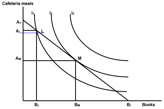
The budget line BL1 shows all the combinations of cafeteria meals and books that Tariq’s limited income will allow him to buy. Tariq maximizes utility by buying the one combination of the commodities in question on the budget line that is tangent to (i.e. just grazes) the highest indifference curve. This provides the highest total utility obtainable given Tariq’s limited income. From the diagram, we observe that the highest achievable indifference curve is I1. The budget restraint is tangent to I1 at point MU. To maximize utility, Tariq should buy BMU of books and CMU of Cafeteria meals. Any other affordable combination (say, N) will be on a lower indifference curve therefore, Tariq will be better off choosing combination MU instead.

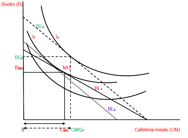
If the price of books falls (to £10) but the price of cafeteria meals remains the same, some changes will be observed on the diagram and there will be what we call, substitution and income effects.

A price change has two notable effects:

1. The substitution effect which arises from the tendency to purchase less of more expensive commodities. This effect can be measured by keeping satisfaction constant…which we can go about by staying on the same indifference curve and finding where Marginal Rate of Substitution (MRS) is = to the new relative price.
2. The income effect arises from the-change in price-effect on the total amount that can be bought. It should also be noted that this effect brings about a change in consumption when we shift to a new indifference curve as a result of the price change. The income effect shows the effect of an increase in real income because there has been a price decrease. This explicitly implies that if the price of a commodity goes down, you can buy more commodities because you now have more purchasing power.

In Tariq’s case (as illustrated by the diagram) when the price of books falls, the budget line pivots. Tariq now maximizes utility by consuming BQ₁ of books and CMQ₁ of cafeteria meals. A fall in the price of books has led to an increase in the quantity demanded of B_MUBQ₁

Now we analyze what happens in a scenario where Tariq’s income falls to £310.

If the prices in commodities, preferences, and tastes of the consumer remain the same and there is a change in income, it will directly affect the consumer’s demand. This effect on the buyer due to an alteration in income is called the income effect. Io our case, Tariq’s income falls and this is illustrated by a shift in the price line downwards to the left (BL_H-BL₂) and he attains lower (tangency) points of equilibrium. However, it should be noted that the shift in the price line is parallel because the prices of the books and cafeteria meals are assumed to remain the same.

Tariq is seen to be back to the same level of utility he was in when he was earning £500 per month. Therefore he is NOT worse off (neither is he better off). This is because, at £310 per month, he can still purchase 12 cafeteria meals and 19 books (because the price of books has fallen to £10). This is illustrated by the price line BL₂ which is still tangent to the original Indifference curve I₁ at a point slightly next to point MU.

Factors that determine the shape of the average cost curves: in the short- run and the long-run And why we might expect economies of scale to be a common occurrence in many firms

Generally, both the Short-run average cost curve and the Long-run average cost curve are characteristically expressed as U-shaped. It should nonetheless be noted that the character of the curves is not a result of identical aspects.

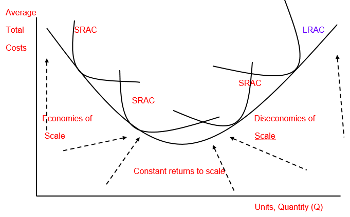
As observed in the diagram above, the long-run average cost (LRAC) curve is an envelope of the short-run average (SRAC) curves. “Also highlighted are the points of increasing, constant and decreasing returns to scale” (Buffet, 2008)

(Buffet, 2008 ) notes “the reasons that bring about the shapes of the average cost curves can be described as follows: In the case of the short-run average curve the initial downward slope is, for the most part, due to declining average fixed costs.” Another factor that plays a role is increasing returns to the variable input at low levels of production. The increasing gradient, on the other hand, is due to decreasing marginal income to the inconsistent input.

“When it comes to the long-run average curve, the shape by definition is a reflection of economies and diseconomies of scale” (Buffet, 2008). At low levels of production, long-run production functions generally display rising returns to scale. For firms that are perfect competitors in input markets, this implies that the long-run average cost is going down. “Continuing, the upward slope of the long-run average cost function at higher levels of output is because of decreasing returns to scale at those specific output levels” (Buffet 2008)

As this organization initially commences to enlarge and open up new plants, it becomes efficient at what it is that it is producing. This way, it can get more output per every unit of input. Consequently, it can experience lower and lower average total costs as it grows bigger. We, therefore, see that “Scale” is synonymous with size. Bringing us to our main concept of ‘Economies of scale’ which stipulates that: “The bigger the firm’s size, the lower its costs of production”, hence, we can expect economies of scale to be a common occurrence in many firms.

References

Buffet, S. N., 2008. Introduction to microeconomics. Dubuque, IA: Kendall Hunt Pub Co.