The Santa Fe Time Series Prediction and Analysis Competition

The desire to predict the future and understand the past drives the search for laws that explain the behaviour of observed phenomena; examples range from the irregularity in a heartbeat to the volatility of a currency exchange rate. If there are known underlying deterministic equations, in principle they can be solved to forecast the outcome of an experiment based on knowledge of the initial conditions.

To make a forecast if the equations are not known, one must find both the rules governing system evolution and the actual state of the system. In this chapter we will focus on phenomena for which underlying equations are not given; the rules that govern the evolution must be inferred from regularities in the past. For example, the motion of a pendulum or the rhythm of the seasons carries within them the potential for predicting their future behaviour from knowledge of their oscillations without requiring insight into the underlying mechanism. We will use the terms understanding” and learning” to refer to two complementary approaches taken to analyze an unfamiliar time series. Understanding is based on explicit mathematical insight into how systems behave, and learning is based on algorithms that can emulate the structure in a time series.

In both cases, the goal is to explain observations; we will not consider the important related problem of using knowledge about a system for controlling it in order to produce some desired behaviour. Time series analysis has three goals: forecasting, modelling, and characterization. The aim of forecasting (also called predicting) is to accurately predict the short-term evolution of the system; the goal of modelling is to find a description that accurately captures features of the long-term behaviour of the system.

These are not necessarily identical: finding governing equations with proper long-term properties may not be the most reliable way to determine parameters for good short-term forecasts, and a model that is useful for short-term forecasts may have incorrect long-term properties. The third goal, system characterization, attempts with little or no a priori knowledge to determine fundamental properties, such as the number of degrees of freedom of a system or the amount of randomness. This overlaps with forecasting but can differ: the complexity of a model useful for forecasting may not be related to the actual complexity of the system. Before the 1920s, forecasting was done by simply extrapolating the series through a global fit in the time domain.

The beginning of modern” time series prediction might be set at 1927 when Yule invented the autoregressive technique in order to predict the annual number of sunspots. His model predicted the next value as a weighted sum of previous observations of the series. In order to obtain interesting behaviour from such a linear system, outside intervention in the form of external shocks must be assumed. For the half-century following Yule, the reigning paradigm remained that of linear models driven by noise.

However, there are simple cases for which this paradigm is inadequate. For example, a simple iterated map, such as the logistic equation (Eq. (11), in Section The Future of Time Series: Learning and Understanding 3 3.2), can generate a broadband power spectrum that cannot be obtained by a linear approximation. The realization that apparently complicated time series can be generated by very simple equations pointed to the need for a more general theoretical framework for time series analysis and prediction. Two crucial developments occurred around 1980; both were enabled by the general availability of powerful computers that permitted much longer time series to be recorded, more complex algorithms to be applied to them, and the data and the results of these algorithms to be interactively visualized.

The first development, state-space reconstruction by time-delay embedding, drew on ideas from differential topology and dynamical systems to provide a technique for recognizing when a time series has been generated by deterministic governing equations and, if so, for understanding the geometrical structure underlying the observed behaviour. The second development was the emergence of the field of machine learning, typified by neural networks, that can adaptively explore a large space of potential models. With the shift in artificial intelligence from rule-based methods towards data-driven methods,[1] the field was ready to apply itself to time series, and time series, now recorded with orders of magnitude more data points than were available previously, were ready to be analyzed with machine-learning techniques requiring relatively large data sets.

The realization of the promise of these two approaches has been hampered by the lack of a general framework for the evaluation of progress. Because time series problems arise in so many disciplines, and because it is much easier to describe an algorithm than to evaluate its accuracy and its relationship to mature techniques, the literature in these areas has become fragmented and somewhat anecdotal. The breadth (and the range in reliability) of relevant material makes it difficult for new research to build on the accumulated insight of past experience (researchers standing on each other’s toes rather than shoulders).

Global computer networks now offer a mechanism for the disjoint communities to attack common problems through the widespread exchange of data and information. In order to foster this process and to help clarify the current state of time series analysis, we organized the Santa Fe Time Series Prediction and Analysis Competition under the auspices of the Santa Fe Institute during the fall of 1991. To explore the results of the competition, a NATO Advanced Research Workshop was held in the spring of 1992; workshop participants included members of the competition advisory board, representatives of the groups that had collected the data, participants in the competition, and interested observers.

Although the participants came from a broad range of disciplines, the discussions were framed by the analysis of common data sets and it was (usually) possible to find a meaningful common ground. In this overview chapter we describe the structure and the results of this competition and review the theoretical material required to understand the successful entries; much more detail is available in the articles by the participants in this volume.

The Competition

The planning for the competition emerged from informal discussions at the Complex Systems Summer School at the Santa Fe Institute in the summer of 1990; the first step was to assemble an advisory board to represent the interests of many of the relevant fields. Second step with the help of this group we gathered roughly 200 megabytes of experimental time series for possible use in the competition. This volume of data reflects the growth of techniques that use enormous data sets (where automatic collection and processing is essential) over traditional time series (such as quarterly economic indicators, where it is possible to develop an intimate relationship with each data point).

In order to be widely accessible, the data needed to be distributed by ftp over the Internet, by electronic mail, and by floppy disks for people without network access. The latter distribution channels limited the size of the competition data to a few megabytes; the final data sets were chosen to span as many of a desired group of attributes as possible given this size limitation (the attributes are shown in Figure 2). The final selection was:

1. A clean physics laboratory experiment. 1,000 points of the fluctuations in a far-infrared laser, approximately described by three coupled nonlinear ordinary deferential equations.
2. Physiological data from a patient with sleep apnea. 34,000 points of the heart rate, chest volume, blood oxygen concentration, and EEG state of a sleeping patient. These observables interact, but the underlying regulatory mechanism is not well understood.
3. High-frequency currency exchange rate data. Ten segments of 3,000 points each of the exchange rate between the Swiss franc and the U.S. Dollar. The average time between two quotes is between one and two minutes.
4. A numerically generated series designed for this competition. A driven particle in a four-dimensional nonlinear multiple-well potential (nine degrees of freedom) with a small non-stationarity drift in the well depths. (Details are given in the Appendix.)
5. Astrophysical data from a variable star. 27,704 points in 17 segments of the time variation of the intensity of a variable white dwarf star, collected by the Whole Earth Telescope (Clemens, this volume). The intensity variation arises from a superposition of relatively independent spherical harmonic multiplets, and there is significant observational noise.

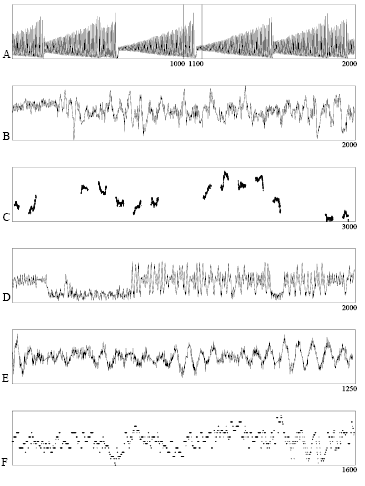
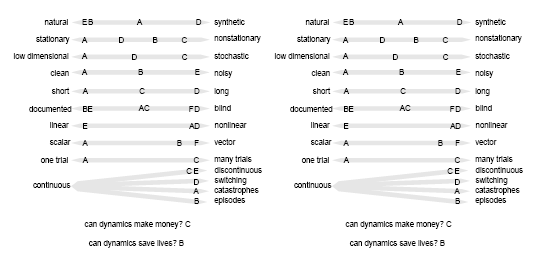
The amount of information available to the entrants about the origin of each data set varied from extensive (Data Sets B and E) to blind (Data Set D). The original files will remain available. The data sets are graphed in Figure 1, and some of the characteristics are summarized in Figure 2. The appropriate level of description for models of these data ranges from low-dimensional stationary dynamics to stochastic processes. After selecting the data sets, we next chose competition tasks appropriate to the data sets and research interests.

The participants were asked to: predict the (withheld) continuations of the data sets with respect to given error measures, characterize the systems (including aspects such as the number of degrees of freedom, predictability, noise characteristics, and the nonlinearity of the system), infer a model of the governing equations, and describe the algorithms employed. The data sets and competition tasks were made publicly available on August 1, 1991, and competition entries were accepted until January 15, 1992.

Participants were required to describe their algorithms. (Insight in some previous competitions was hampered by the acceptance of proprietary techniques.) One interesting trend in the entries was the focus on prediction, for which three motivations were given:

1. because predictions are falsifiable, insight into a model used for prediction is verifiable;
2. there are a variety of financial incentives to study prediction; and
3. the growth of interest in machine learning brings with it the hope that there can be universally and easily applicable algorithms that can be used to generate forecasts.

Another trend was the general failure of simplistic black box” approaches in all successful entries, exploratory data analysis preceded the algorithm application.

It is interesting to compare this time series competition to the previous state of the art as reflected in two earlier competitions. In these, a very large number of time series was provided (111 and 1001, respectively), taken from business (forecasting sales), economics (predicting recovery from the recession), finance, and the social sciences. However, all of the series used were very short, generally less than 100 values long. Most of the algorithms entered were fully automated, and most of the discussion centered around linear models.[4] In the Santa Fe Competition all of the successful entries were fundamentally nonlinear and, even though significantly more computer power was used to analyze the larger data sets with more complex models, the application of the algorithms required more careful manual control than in the past.

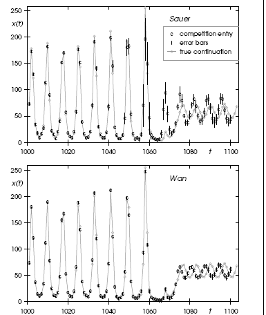
Wan. Predicted values are indicated by “c,” predicted error bars by vertical lines. The true continuation (not available at the time when the predictions were received) is shown in grey (the points are connected to guide the eye).

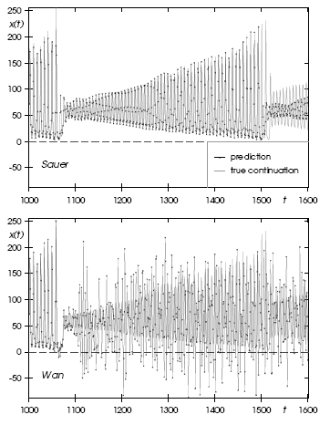
Figure 4 Predictions obtained by the same two models as in the previous figure, but continued 500 points further into the future. The solid line connects the predicted points; the grey line indicates the true continuation.

As an example of the results, consider the intensity of the laser (Data Set A; see Figure 1). On the one hand, the laser can be described by a relatively simple correct” model of three nonlinear deferential equations, the same equations that Lorenz (1963) used to approximate weather phenomena. On the other hand, since the 1,000-point training set showed only three of four collapses, it is difficult to predict the next collapse based on so few instances. For this data set we asked for predictions of the next 100 points as well as estimates of the error bars associated with these predictions. We used two measures to evaluate the submissions.

The first measure (normalized mean squared error) was based on the predicted values only; the second measure used the submitted error predictions to compute the likelihood of the observed data given the predictions. The Appendix to this chapter gives the definitions and explanations of the error measures as well as a table of all entries received. We would like to point out a few interesting features. Although this single trial does not permit fine distinctions to be made between techniques with comparable performance, two techniques clearly did much better than the others for Data Set A; one used state-space reconstruction to build an explicit model for the dynamics and the other used a connectionist network (also called a neural network).

Incidentally, a prediction based solely on visually examining and extrapolating the training data did much worse than the best techniques, but also much better than the worst. Figure 3 shows the two best predictions. Sauer (this volume) attempts to understand and develop a representation for the geometry in the system’s state space, which is the best that can be done without knowing something about the system’s governing equations, while Wan (this volume) addresses the issue of function approximation by using a connectionist network to learn to emulate the input-output behaviour. Both methods generated remarkably accurate predictions for the specified task.

In terms of the measures defined for the competition, Wan’s squared errors are one-third as large as Sauer’s, and taking the predicted uncertainty into account Wan’s model is four times more likely than Sauer’s. According to the competition scores for Data Set A, this puts Wan’s network in the first place. A different picture, which cautions the hurried researcher against declaring one method to be universally superior to another, emerges when one examines the evolution of these two prediction methods further into the future. Figure 4 shows the same two predictors, but now the continuations extend 500 points beyond the 100 points submitted for the competition entry (no error estimates are shown).

The neural network’s class of potential behaviour is much broader than what can be generated from a small set of coupled ordinary differential equations, but the state-space model is able to reliably forecast the data much further because its explicit description can correctly capture the character of the long-term dynamics. In order to understand the details of these approaches, we will detour to review the framework for (and then the failure of) linear time series analysis.

Linear Time Series Models

Linear time series models have two particularly desirable features: they can be understood in great detail and they are straightforward to implement. The penalty for this convenience is that they may be entirely inappropriate for even moderately complicated systems. In this section we will review their basic features and then consider why and how such models fail. The literature on linear time series analysis is vast; a good introduction is the very readable book by Chatfield (1989), many derivations can be found (and understood) in the comprehensive text by Priestley

(1981), and a classic reference is Box and Jenkins’ book (1976). Historically, the general theory of linear predictors can be traced back to Kolmogorov (1941) and to Wiener (1949). Two crucial assumptions will be made in this section: the system is assumed to be linear and stationary. In the rest of this chapter we will say a great deal about relaxing the assumption of linearity; much less is known about models that have coefficients that vary with time. To be precise, unless explicitly stated (such as for Data Set D), we assume that the underlying equations do not change in time, i.e., time invariance of the system.

Arma, Fir, and All That

There are two complementary tasks that need to be discussed: understanding how a given model behaves and finding a particular model that is appropriate for a given time series. We start with the former task. It is simplest to discuss separately the role of external inputs (moving average models) and internal memory (autoregressive models).

Properties of a Given Linear Model

Moving average (MA) models. Assume we are given an external input series {e_t} and want to modify it to produce another series {x_t}. Assuming linearity of the system and causality (the present value of x is influenced by the present and N past values of the input series e), the relationship between the input and output is

This equation describes a convolution filter: the new series x is generated by an Nth-order filter with coefficients b_{0……………….}b_n from the series e. Statisticians and econometricians call this an Nth-order moving average model, MA(N). The origin of this (sometimes confusing) terminology can be seen if one pictures a simple smoothing filter which averages the last few values of series e. Engineers call this a finite impulse response (FIR) filter, because the output is guaranteed to go to zero at N time steps after the input becomes zero. Properties of the output series x clearly depend on the input series e. The question is whether there are characteristic features independent of a specific input sequence. For a linear system, the response of the filter is independent of the input. A characterization focuses on properties of the system, rather than on properties of the time series. (For example, it does not make sense to attribute linearity to a time series itself, only to a system.)

We will give three equivalent characterizations of an MA model: in the time domain (the impulse response of the filter), in the frequency domain (its spectrum), and in terms of its autocorrelation coefficients. In the first case, we assume that the input is nonzero only at a single time step t0 and that it vanishes for all other times. The response (in the time domain) to this impulse” is simply given by the b’s in Eq. (1): at each time step the impulse moves up to the next coefficient until, after N steps, the output disappears. The series b_N,b_N-1……………. b0 is thus the impulse response of the system.

The response to an arbitrary input can be computed by superimposing the responses at appropriate delays, weighted by the respective input values (convolution”). The transfer function thus completely describes a linear system, i.e., a system where the superposition principle holds: the output is determined by impulse response and input. Sometimes it is more convenient to describe the filter in the frequency domain. This is useful (and simple) because a convolution in the time domain becomes a product in the frequency domain. If the input to a MA model is an impulse (which has a flat power spectrum), the discrete Fourier transform of the output is given by

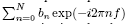
(see, for example, Box & Jenkins, 1976, p.69). The power spectrum is given by the squared magnitude of this:

The third way of representing yet again the same information is, in terms of the autocorrelation coefficients, defined in terms of the mean µ = x{t} and the

Variance σ² = [{ X_t – µ ² }]

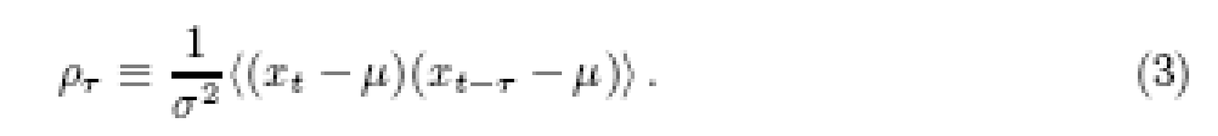
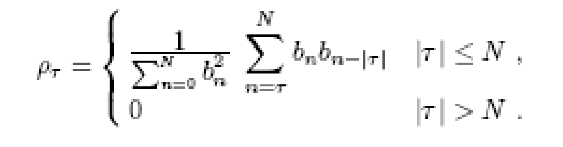
The autocorrelation coefficients describe how much, on average, two values of a series that are ζ time steps apart co-vary with each other. (We will later replace this linear measure with mutual information, suited also to describe nonlinear relations.) If the input to the system is a stochastic process with input values at different times uncorrelated, {e_i e_j} = 0 or i not equal to j, then all of the cross terms will disappear from the expectation value in Eq. (3), and the resulting autocorrelation coefficients are

The Breakdown of Linear Models

We have seen that ARMA coefficients, power spectra, and autocorrelation coefficients contain the same information about a linear system that is driven by uncorrelated white noise. Thus, if and only if the power spectrum is a useful characterization of the relevant features of a time series, an ARMA model will be a good choice for describing it. This appealing simplicity can fail entirely for even simple nonlinearities if they lead to complicated power spectra (as they can). Two time series can have very similar broadband spectra but can be generated from systems with very different properties, such as a linear system that is driven stochastically by external noise, and a deterministic (noise-free) nonlinear system with a small number of degrees of freedom. One the key problems addressed in this chapter is how these cases can be distinguished linear operators definitely will not be able to do the job.

Let us consider two nonlinear examples of discrete-time maps (like an AR model, but now nonlinear):

The first example can be traced back to Ulam (1957): the next value of a series is derived from the present one by a simple parabola

Popularized in the context of population dynamics as an example of a simple mathematical model with very complicated dynamics” (May, 1976), it has been found to describe a number of controlled laboratory systems such as hydrodynamic flows and chemical reactions, because of the universality of smooth unimodal maps (Collet, 1980). In this context, this parabola is called the logistic map or quadratic map. The value xt deterministically depends on the previous value xt-1 ; λ ¸ is a parameter that controls the qualitative behaviour, ranging from a fixed point (for small values of ) to deterministic chaos. For example, for λ = 4, each iteration destroys one bit of information.

Consider that, by plotting xt against xt-1, each value of xt has two equally likely predecessors or, equally well, the average slope (its absolute value) is two: if we know the location within before the iteration, we will on average know it within 2e afterwards. This exponential increase in uncertainty is the hallmark of deterministic chaos (divergence of nearby trajectories”). The second example is equally simple: consider the time series generated by the map

Understanding and Learning

Strong models have strong assumptions. They are usually expressed in a few equations with a few parameters, and can often explain a plethora of phenomena. In weak models, on the other hand, there are only a few domain-specific assumptions. To compensate for the lack of explicit knowledge, weak models usually contain many more parameters (which can make a clear interpretation difficult). It can be helpful to conceptualize models in the two-dimensional space spanned by the axes data-poor data-rich and theory-poor theory-rich. Due to the dramatic expansion of the capability for automatic data acquisition and processing, it is increasingly feasible to venture into the theory-poor and data-rich domain.

Strong models are clearly preferable, but they often originate in weak models. (However, if the behaviour of an observed system does not arise from simple rules, they may not be appropriate.) Consider planetary motion (Gingerich, 1992). Tycho Brahe’s (1546{1601) experimental observations of planetary motion were accurately described by Johannes Kepler’s (1571{1630) phenomenological laws; this success helped lead to Isaac Newton’s (1642{1727) simpler but much more general theory of gravity which could derive these laws; Henri Poincar¶e’s (1854{1912) inability to solve the resulting three-body gravitational problem helped lead to the modern theory of dynamical systems and, ultimately, to the identification of chaotic planetary motion (Busman & Wisdom, 1988, 1992).

As in the previous section on linear systems, there are two complementary tasks: discovering the properties of a time series generated from a given model, and inferring a model from observed data. We focus here on the latter, but there has been comparable progress for the former. Exploring the behaviour of a model has become feasible in interactive computer environments, such as Cornell’s dstool,[9] and the combination of traditional numerical algorithms with algebraic, geometric, symbolic, and artificial intelligence techniques is leading to automated platforms for exploring dynamics (Abelson’s, 1990; Yip, 1991; Bradley, 1992).

For a nonlinear system, it is no longer possible to decompose an output into an input signal and an independent transfer function (and thereby find the correct input signal to produce a desired output), but there are adaptive techniques for controlling nonlinear systems (Hauler, 1989; Tot, Grebe & Yorke, 1990) that make use of techniques similar to the modelling methods that we will describe. The idea of weak modelling (data-rich and theory-poor) is by no means new| an ARMA model is a good example.

What is new is the emergence of weak models (such as neural networks) that combine broad generality with insight into how to manage their complexity. For such models with broad approximation abilities and few specific assumptions, the distinction between memorization and generalization becomes important. Whereas the signal-processing community sometimes uses the available by anonymous ftp from macomb.tn.cornell.edu in pub/stool. The Future of Time Series:

Learning and Understanding term learning for any adaptation of parameters, we need to contrast learning without generalization from learning with generalization. Let us consider the widely and wildly celebrated fact that neural networks can learn to implement the exclusive OR (XOR). But what kind of learning is this? When four out of four cases are specified, no generalization exists! Learning a truth table is nothing but rote memorization: learning XOR is as interesting as memorizing the phone book. More interesting and more realistic are real-world problems, such as the prediction of financial data. In forecasting, nobody cares how well a model fits the training data| only the quality of future predictions counts, i.e., the performance on novel data or the generalization ability.

Learning means extracting regularities from training examples that do transfer to new examples. Learning procedures are, in essence, statistical devices for performing inductive inference. There is a tension between two goals. The immediate goal is to ¯t the training examples, suggesting devices as general as possible so that they can learn a broad range of problems. In connectionism, this suggests large and flexible networks, since networks that are too small might not have the complexity needed to model the data. The ultimate goal of an inductive device is, however, its performance on cases it has not yet seen, i.e., the quality of its predictions outside the training set.

This suggests at least for noisy training data networks that are not too large since networks with too many high-precision weights will pick out idiosyncrasies of the training set and will not generalize well. An instructive example is polynomial curve fitting in the presence of noise. On the one hand, a polynomial of too low an order cannot capture the structure present in the data. On the other hand, a polynomial of too high an order, going through all of the training points and merely interpolating between them, captures the noise as well as the signal and is likely to be a very poor predictor for new cases. This problem of fitting the noise in addition to the signal is called over fitting.

By employing a regularizer (i.e., a term that penalizes the complexity of the model) it is often possible to ¯t the parameters and to select the relevant variables at the same time. Neural networks, for example, can be cast in such a Bayesian framework (Buntine & Weigend, 1991). To clearly separate memorization from generalization, the true continuation of the competition data was kept secret until the deadline, ensuring that the continuation data could not be used by the participants for tasks such as parameter estimation or model selection.

Successful forecasts of the withheld test set (also called out-of-sample predictions) from the provided training set (also called fitting set) were produced by two general classes of techniques: those based on state space reconstruction (which make use of explicit understanding of the relationship between the internal degrees of freedom of a deterministic system and an observable of the system’s state in order to build a model of the rules governing the measured behaviour of the system), and connectionist modelling (which uses potentially rich models along with learning algorithms to develop an implicit model of the system). We will see that neither is uniquely preferable. The domains of applicability are not the same, and the choice of which to use depends on the goals of the analysis (such as an understandable description vs. Accurate short-term forecasts).

The Future

We have surveyed the results of what appears to be a steady progress of insight over ignorance in analyzing time series. Is there a limit to this development? Can we hope for the discovery of a universal forecasting algorithm that will predict everything about all time series? The answer is emphatically no!” Even for completely deterministic systems, there are strong bounds on what can be known. The search for a universal time series algorithm is related to Hilbert’s vision of reducing all of mathematics to a set of axioms and a decision procedure to test the truth of assertions based on the axioms (Entscheidungs problem); this culminating dream of mathematical research was dramatically dashed by Gödel (1931) and then by Turing.

The most familiar result of Turing is the undecidability of the halting problem: it is not possible to decide in advance whether a given computer program will eventually halt (Turing, 1936). But since Turing machines can be implemented with dynamical systems (Fredkin, 1982; Moore, 1991), a universal algorithm that can directly forecast the value of a time series at any future time would need to contain a solution to the halting problem, because it would be able to predict whether a program will eventually halt by examining the program’s output. Therefore, there cannot be a universal forecasting algorithm.

The connection between computability and time series goes deeper than this.

The invention of Turing machines and the undecidability of the halting problem were side results of Turing’s proof of the existence of uncomputable real numbers.

Unlike a number such as ¼, for which there is a rule to calculate successive digits, he showed that there are numbers for which there cannot be a rule to generate their digits. If one was unlucky enough to encounter a deterministic time series generated by a chaotic system with an initial condition that was an uncomputable real number, then the chaotic dynamics would continuously reveal more and more digits of this number. Correctly forecasting the time series would require calculating unseen digits from the observed ones, which is an impossible task. Perhaps we can be more modest in our aspirations. Instead of seeking complete future knowledge from present observations, a more realistic goal is to find the best model for the data, and a natural definition of best” is the model that requires the least amount of information to describe it. This is exactly the aim of

Algorithmic Information Theory, independently developed by Chaitin (1966), Kolmogorov (1965), and Solomono® (1964). Classical information theory, described in Section 6.2, measures information with respect to a probability distribution of an ensemble of observations of a string of symbols. In algorithmic information theory, information is measured within a single string of symbols by the number of bits needed to specify the shortest algorithm that can generate them. This has led to significant extensions of Gaodel and Turing’s results (Chaitin, 1990) and, through

Hofstadter paraphrases Gaodel’s Theorem as: All consistent axiomatic formulations of number theory include undecidable propositions.” (Hofstadter, 1979, p. 17).

The Future of Time Series: Learning and Understanding 61 the Minimum Description Length principle, it has been used as the basis for a general theory of statistical inference (Wallace & Boulton, 1968; Rissanen, 1986, 1987). Unfortunately, here again we run afoul of the halting problem. There can be no universal algorithm to find the shortest program to generate an observed sequence because we cannot determine whether an arbitrary candidate program will continue to produce symbols or will stop.

Questionnaire

Whether the daily returns of the US exchange rate data with the individual countries exhibit time series stationarity

Answer Eastern Asian countries experienced rapid economic growth and were fast becoming prosperous if not booming economies. Average economic growth of Thailand, Malaysia, Indonesia and South Korea ranged from 6.9% to 8.4%. The ASEAN group countries (Thailand, Malaysia, Indonesia, Singapore and Philippines) attracted vast capital inflows, accounting for more then half of all the capital inflows into developing countries. The revolution of these less developed countries into middle income or emerging economies was seen as a “remarkable historical achievement”, and was called the ‘Asian Miracle’ (Stanley Fischer).

The crisis were caused by a “knock on effect” or “domino effect” of the Thai crisis, or whether they were due to inherent instability of the exchange rates and macroeconomic policies of the other countries in the South East Asia region would depend upon how the researcher perceived the question and the null hypothesis being tested as well which data considered relevant to include in the model. One school of thought, as postulated by Andrew Berg is that the crisis was due to macroeconomic mismanagement, however Copeland questions this thesis, although the conditions might be suitable for an exchange rate collapse, theory is unable to predict such crises.

Whether the daily returns were co integrated before and after the crisis?

Answer The Asian financial crisis, described by Chang Ha-Joon in his book as starting in Thailand, resulting in a forty percent devaluation of the Thailand Baht against the US dollar, and spread on to Indonesia, Malaysia and Philippines causing devaluations of up to sixty percent, with devastating repercussions on the economic stability and growth impacting for years after the event. Andrew Berg in the paper “The Asian Crisis: Causes, Policy Responses and Outcomes” claims that the crisis was generally perceived as being due to “authorities left without effective tools to counter sudden capital outflows. The pattern of output decline suggests that these vulnerabilities, particularly weaknesses in domestic financial system, played a larger role than tight monetary policy in determining outcomes”, suggesting that the crisis was caused by poor macroeconomic management combined with the decision to float the baht in international exchange markets.

“The crisis had their origins in fundamental deficiencies in the affected countries. In Thailand, some role was played by traditional macroeconomic problems, particularly current account deficits that became unsustainably large and an exchange rate that had become overvalued. Generally, though, the weaknesses in the crisis countries derived from the interaction of weak domestic financial institutions with large capital inflows. According to this interpretation, over investing in poor projects resulted from pervasive moral hazard problems in domestic financial institutions and perhaps poor lending practices among creditors” (Berg 1999).

Whether there was an identifiable GARCH pattern to the volatility of daily returns of the individual currencies?

Answer It is well-established that the volatility of asset prices displays considerable persistence. That is, large movements in prices tend to be followed by more large moves, producing positive serial correlation in squared returns. Thus current and past volatility can be used to predict future volatility. This fact is important to both financial market practitioners and regulators. Professional traders in equity and foreign exchange markets must pay attention not only to the expected return from their trading activity but also to the risk that they incur. Risk averse investors will wish to reduce their exposure during periods of high volatility and improvements in risk-adjusted performance depend upon the accuracy of volatility predictions.

Many current models of risk management, such as Value-at-Risk (VaR), use volatility predictions as inputs. The bank capital adequacy standards recently proposed by the Basle Committee on banking supervision illustrate the importance of sophisticated risk management techniques for regulators. These norms are aimed at providing international banks with greater incentives to manage financial risk in a sophisticated fashion, so that they might economize on capital.

One such system that is widely used is Risk Metrics, developed by J.P. Morgan. A core component of the Risk Metrics system is a statistical model—a member of the large ARCH/GARCH family—that forecasts volatility. Such ARCH/GARCH models are parametric. That is, they make specific assumptions about the functional form of the data generation process and the distribution of error terms.

Parametric models such as GARCH are easy to estimate and readily interpretable, but these advantages may come at a cost. Other, perhaps much more complex models may be better representations of the underlying data generation process. If so, then procedures designed to identify these alternative models have an obvious payoff. Such procedures are described as non-parametric. Instead of specifying a particular functional form for the data generation process and making distributional assumptions about the error terms, a non-parametric procedure will search for the best fit over a large set of alternative functional forms.

This article investigates the performance of a genetic program applied to the problem of forecasting volatility in the foreign exchange market. Genetic programming is a computer search and problem-solving methodology that can be adapted for use in non-parametric estimation. It has been shown to detect patterns in the conditional mean of foreign exchange and equity returns that are not accounted for by standard statistical models (Neely, Weller, and Dittmar 1997; Neely and Weller 1999 and 2001; Neely 2000). These models are widely used both by academics and practitioners and thus are good benchmarks to which to compare the genetic program forecasts. While the overall forecast performance of the two methods is broadly similar, on some dimensions the genetic program produces significantly superior results. This is an encouraging finding, and suggests that more detailed investigation of this methodology applied to volatility forecasting would be warranted.

References

1. Abelson, H. 1990. The Bifurcation Interpreter: A Step Towards the Automatic Analysis of Dynamical Systems.” Intl. J. Comp. & Math. Appl. 20:13.
2. Afraimovich, V. S., M. I. Rabinovich, and A. L. Zheleznyak. 1993. Finite-Dimensional Spatial Disorder: Description and Analysis.” In Time Series Prediction: Forecasting the Future and Understanding the Past, edited by A. S. Weigend and N. A. Gershenfeld, 539{556. Reading, MA: Addison-Wesley.
3. Akaike, H. 1970. Statistical Predictor Identi¯cation.” Ann. Inst. Stat. Math. 22: 203{217.
4. Alesic, Z. 1991. Estimating the Embedding Dimension.” Physica D 52: 362{368.
5. Barron, A. R 1993 Universal Approximation Bounds for Superpositions of a Sigmoidal Function.” IEEE Trans. Info. Theory 39(3): 930{945.
6. Beck, C. 1990. Upper and Lower Bounds on the Renyi Dimensions and the Uniformity of Multifractals.” Physica D 41: 67{78.
7. Broomhead, D. S., and D. Lowe. 1988. Multivariable Functional Interpolation and Adaptive Networks.” Complex Systems 2: 321{355.
8. Brown, R., P. Bryant, and H. D. I. Abarbanel. 1991. Computing the Lyapunov Spectrum of Dynamical System from an Observed Time Series.” Phys. Rev. A 43: 2787{806.
9. Buntine, W. L., and A. S. Weigend. 1991. Bayesian Backpropagation.” Complex Systems 5: 603{643.
10. Casdagli, M. 1989. Nonlinear Prediction of Chaotic Time Series.” Physica D 35: 335{356.
11. Casdagli, M. 1991. Chaos and Deterministic versus Stochastic Nonlinear Modeling.” J. Roy. Stat. Soc. B 54: 303{328.
12. Casdagli, M., S. Eubank, J. D. Farmer, and J. Gibson. 1991. State Space Reconstruction in the Presence of Noise.” Physica D 51D: 52{98.
13. Casdagli, M. C., and A. S. Weigend. 1993. Exploring the Continuum Between Deterministic and Stochastic Modeling.” In Time Series Prediction: Forecasting the Future and Understanding the Past, edited by A. S. Weigend and N. A. Gershenfeld, 347-366. Reading, MA: Addison-Wesley.
14. Catlin, D. E. 1989. Estimation, Control, and the Discrete Kalman Filter. Applied Mathematica Sciences, Vol. 71. New York: Springer-Verlag, 1989.
15. Chaitin, G. J. 1966. On the Length of Programs for Computing Finite Binary Sequences.” J. Assoc. Comp. Mach 13: 547{569.
16. Chaitin, G. J. 1990. Information, Randomness Incompleteness. Series in Computer Science, Vol. 8, 2nd ed. Singapore: World-Scienti¯c.
17. Chatfield, C. 1988. What is the Best Method in Forecasting?” J. Appl. Stat. 15: 19{38.
18. Lewis, P. A. W., B. K. Ray, and J. G. Stevens. 1993. Modeling Time Using Multivariate Adaptive Regression Splines (MARS).” In Time Series Prediction: Forecasting the Future and Understanding the Past, edited Weigend and N. A. Gershenfeld, 296-318. Reading, MA: Addison-Wesley.
19. Liebert, W., and H. G. Schuster. 1989. Proper Choice of the Time Delay Analysis of Chaotic Time Series.” Phys. Lett. A 142: 107{111.
20. Lorenz, E. N. 1963. Deterministic Non-Periodic Flow.” J. Atmos. Sci. 141.
21. Lorenz, E. N. 1989. Computational Chaos|A Prelude to Computational Instability.” Physica D 35: 299{317.
22. Makridakis, S., A. Andersen, R. Carbone, R. Fildes, M. Hibon, R. Lewandowski, J. Newton, E. Parzen, and R. Winkler. 1984. The Forecasting Accuracy Major Time Series Methods. New York: Wiley.
23. Makridakis, S., and M. Hibon. 1979. Accuracy of Forecasting: An Empirical Investigation.” J. Roy. Stat. Soc. A 142: 97{145. With discussion.
24. Marteau, P. F., and H. D. I. Abarbanel. 1991. Noise Reduction in Chaotic Series Using Scaled Probabilistic Methods.” J. Nonlinear Sci. 1: 313. R. M. 1976. Simple Mathematical Models with Very Complicated Dynamics.” Nature 261: 459.
25. Melvin, P., and N. B. Tu¯llaro. 1991. Templates and Framed Braids.” Phys. A 44: R3419{R3422.
26. Meyer, T. P., and N. H. Packard. 1992. Local Forecasting of High-Dimensional Chaotic Dynamics.” In Nonlinear Modeling and Forecasting, edited by Casdagli and S. Eubank. Santa Fe Institute Studies in the Sciences of Complexity, Proc. Vol. XII, 249{263. Reading, MA: Addison-Wesley.
27. Rissanen, J. 1987. Stochastic Complexity.” J. Roy. Stat. Soc. B 49: 223{239. With discussion: 252{265.
28. Ruelle, D., and J. P. Eckmann. 1985. Ergodic Theory of Chaos and Strange Attractors.” Rev. Mod. Phys. 57: 617{656.
29. Sakamoto, Y., M. Ishiguro, and G. Kitagawa. 1986. Akaike Information Criterion Statistics. Dordrecht: D. Reidel.
30. Sauer, T. 1992. A Noise Reduction Method for Signals from Nonlinear Systems.” Physica D 58: 193{201.
31. Sauer, T. 1993. Time Series Prediction Using Delay Coordinate Embedding.” In Time Series Prediction: Forecasting the Future and Understanding the Past, edited by A. S. Weigend and N. A. Gershenfeld, 175{193. Reading, MA: Addison-Wesley.