Significant of meeting assumptions in statistical test
In a statistical analysis, assumptions made are very significant in designing of the research method applicable to a given case scenario. Ensuring that the data meets a given assumption helps in reducing the errors during computation, particularly type one and two errors. The assumptions help in boosting the reliability, avoided non-normality, reduce cases of curvilinearity and consequently, give an output which is desirable. The assumptions ease the performance of the parametric tests and therefore, are in a position to effectively and efficiently compute the output.
Histograms with normal curves
Probability plots (p-p plots)
Examination of normality
The probability plots shown above indicate that the hygiene variable for day 1 displays a normal distribution where the largest probability was recorded at the centre and reduced to the ends. The hygiene variable for days 2 and day 3 shows that there is a slight shift of the most concentrated values towards the left side and therefore, this is where a normality assumption comes into being.
Descriptive analysis
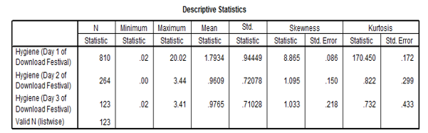
The above shows the measures of central tendencies. From the values given, the hygiene for day one is not normally distributed since there is a great variation in the differences between the minimum and the mean and the maximum and the mean. The hygiene variables for day 2 and three shows that their data is normally distributed by the virtue that the mean lies almost at the middle of the maximum and the minimum values (Field, 2009).
The skewness of the data which is a measure of how the data is distributed towards the right or the left of the mean shows that for day 1 the data is skewed more to the right contrary to the probability plots. The skewness of the hygiene for day 2 and 3 are skewed to the right but by a very small margin.
Kurtosis which is the level of flatness of the data shows that the hygiene for day one is more peaked at the centre as compared with the other two variables which are more flattened.
Descriptive analysis for SPSS Exam
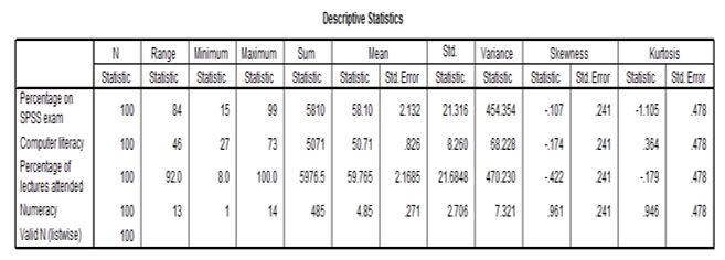
The above table shows the descriptive analysis with the measures of central tendencies. The skewness shows that the variables are skewed by small value to the right which is less than one in both cases. This is an indication that the data has its values gradually decreasing from the mean. The kurtosis analysis shows that the values are fairly flat and there is no significant sharp increase in the variables at the centre or the mean.
Figure 7, 8, 9 and 10 shows the histograms for the variables in the data set. It is clear that figure 8 and 9 which represents the literacy and the percentage of the lecturers attended shows that the values fairly follow the normal curve where the value is highest at the middle and decreases to the right and the left. In this case, we can conclude that the data has a normal distribution basing on the graphs. Which is for the percentage on the SPSS exam do not follow the normal distribution at all. The values are randomly distributed, and it is not conclusive where the data is skewed towards whether it is to the left or the right. On the other hand, figure 10 shows that the numeracy variable shows that the values are skewed to the left and decreases to the right.
Test for homogeneity of variance
Test of Homogeneity of Variances.
ANOVA
The above Levene’s test also known as the ANOVA test shows that the percentage of the lecturers who meets the criteria set for the homogeneity of variance is 2.584, which suggests that the largest variance should be at most four times the smallest value of variance. Therefore, this condition is satisfied hence the data has homogeneity of variance (Field, 2009).
Assumptions of normality and homogeneity of variance
The assumption of normality means that the data is assumed to be distributed about the mean where most of the data are concentrated at the centre and reduces towards the extremes. On the other hand, the assumptions of covariance mean that the variance of the variables should not differ by a large margin. The largest variance should be four times for the smallest variance for this assumption to be adhered. In situations where this assumption is violated, it leads to false conclusions from a given set of data. There are situations where the effects are not felt, for instance, when a larger number of responses is nearly equal or equal to the mean.
The violation can be addressed by transformation of data, using a more conservative ANOVA test, using tests, which are free from distribution issues and trimming the data to fit the normal distribution.
Reference
Field, A. (2009). Discovering statistics using SPSS (3rd ed.). Los Angeles: Sage.