Introduction
In science, it is paramount to be able to analyze data in order to discover correlations between phenomena (Campbell & Stanley, 1963). This paper provides a multiple regression analysis of the data for the task 4 of the textbook by Field (2013, p. 355); the data can be found in the file “supermodel.sav” on the “Datasets” (n.d.) webpage. In the paper, the assumptions for the multiple regression are discussed and tested; their violations are addressed. After that, the hypotheses for the test are provided. Finally, the results of the tests are supplied. It is also explained how to achieve the power of.8 for the test at α=.05 and with the appropriate effect size. The SPSS output can be found in appendices.
Underlying Assumptions for a Multiple Regression
The assumptions for a multiple regression are as follows (Warner, 2013; Field, 2013):
- The dependent variable ought to be quantitative, and the distribution of its values should be close to normal; (assessed by looking at univariate distribution)
- The independent variables also ought to be quantitative and their distribution should approximate the normal one; however, they can be dichotomous or dummy;
- The individual observations should not be correlated;
- Each independent variable should have a correlation to the dependent variable which approximates the linear relation;
- There needs to be homogeneity of variances (homoscedasticity) of the values of the dependent variable across levels of each of the independent variables;
- No multicollinearity (high correlation between any two independent variables) should exist in the data.
Testing the Assumptions and Addressing their Violations
Assumption 1. The dependent variable (salary) is quantitative. The distribution of its values can be assessed by using a histogram:
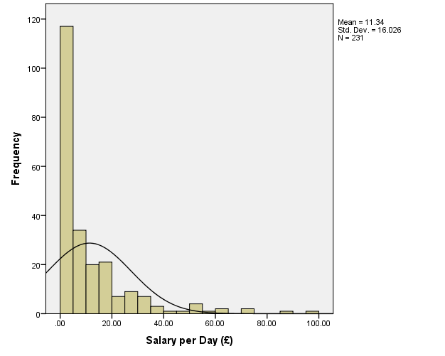
Unfortunately, the distribution has many values close to 0, which makes it “peaked” (the kurtosis is likely to be positive), and there are a large number of extreme outliers with z>2.5, which makes the model unacceptable (Field, 2013).
To address this problem, the outliers with z>2.5 for the current distribution, i.e. the cases where salary is higher than approximately £51, will be removed from the sample. However, the examination of the data revealed that there is a value of salary=48.87 (case #24), and it is likely that this will be a new extreme outlier in the modified data (it can also be seen at the histogram above together with salary=51.03 at #41). Therefore, the values where salary is higher than £48 will be get rid of. This results in the following distribution:
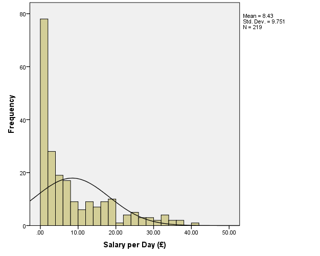
There is a new outlier salary=41.05 at #83, but it will be left in the sample; in addition, it is stated that such an outlier is acceptable (Field, 2013).
Next, it might be needed to address the large number of values where salary is approximately between 0 and 2, which results in non-normality. It is possible to deal with this by raising the values of the salary variable to a certain power. In this case, the power of.25 will be used. The result is as follows:
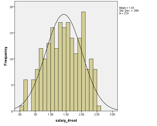
It is easy to see that the resulting variable salary_4root is much closer to a normally distributed variable than the original salary variable. Thus, in the following procedures, the variable salary_4root will be used instead of salary.
Assumption 2. The rest of the variables are approximately normally distributed, as can be seen from the histograms:
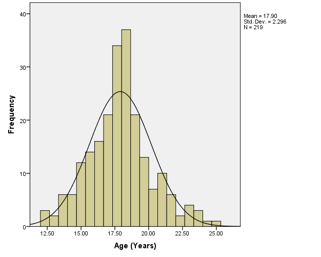
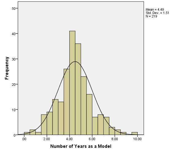
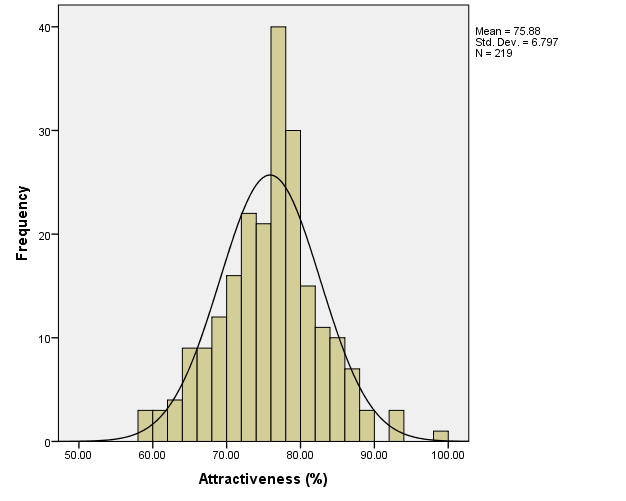
Similarly to the salary variable, if the values of these variables were not normally distributed, it would be possible to apply transformations to them, for instance, by raising them to certain powers. Extreme outliers could be dealt with by removing them from calculations, also similarly to what was done with the salary variable.
Assumption 3. The individual observations are not correlated, for the salaries, attractiveness, age and experience of the different models are not correlated. If the assumption was violated, it would be important to remove the correlated observations from the sample.
Assumption 4. To find out whether there are linear correlations between the dependent variable and the independent variables, it is possible to examine the scatter plots:
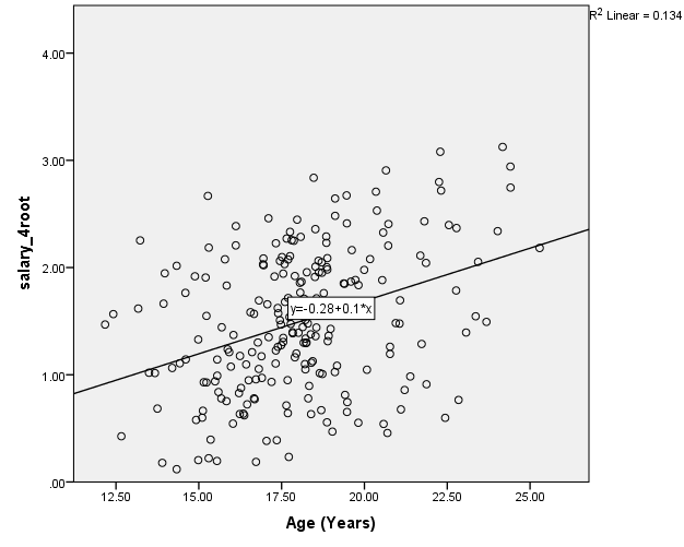
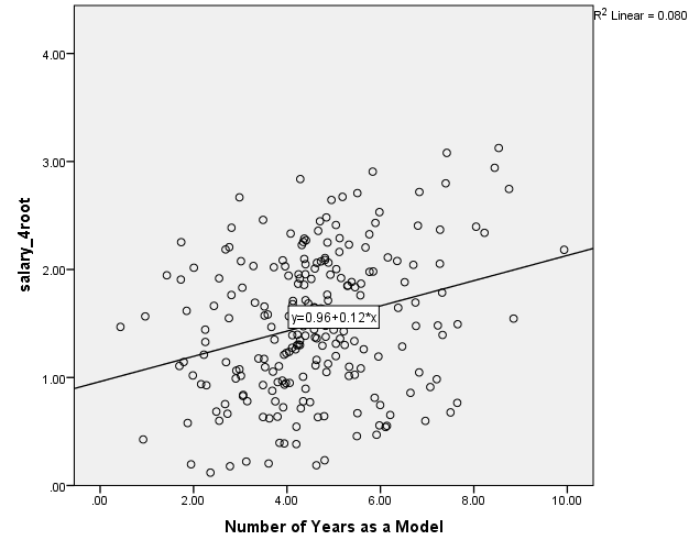
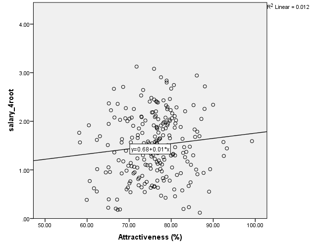
It can be seen that, among the variables, the strongest correlation is between the age and salary_4root variables: the coefficient of determination is R2=.134; therefore, the correlation coefficient is r=.366. There is a weaker correlation between years and salary_4root, R2=.080, r=.283. Also, there is almost no correlation between the beauty and salary_4root, R2=.012, r=.110.
Assumption 5. Homoscedasticity can be tested by using a scatter plot of standardized residuals vs. standardized predicted values (zresid vs. zpred) (Field, 2013). The plot is as follows:
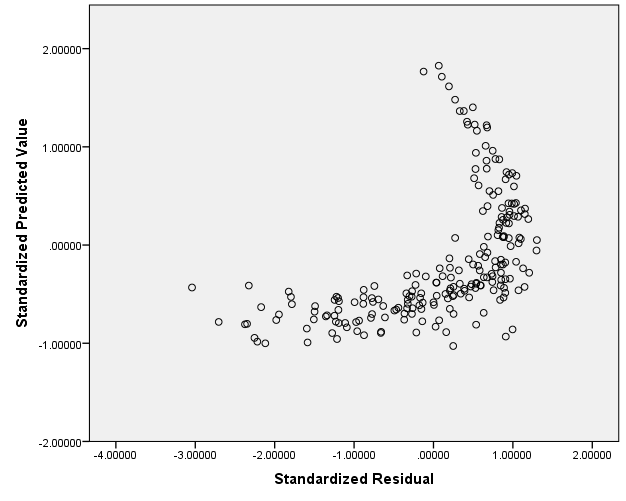
Such a plot is characteristic of data which satisfies the assumption of homoscedasticity. (The violation of this assumption can be addressed by logarithmic or square root data transformations.)
On the other hand, because there is a curve on the plot, it shows that the assumption of linearity may be violated. It can also be addressed by using data transformation. However, because the “upper” part of the scatter plot is “thin,” that is, it only includes a small number of data points, it might be possible to run a multiple regression without further alterations of the data.
Assumption 6. Multiocollinearity can be tested by repeatedly running linear regressions which use one of the independent variables as a dependent variable in turn. The results of these can be found in Appendix 1. As it can be seen, the variables age and years are highly collinear (VIF = 10.036). This should be expected, because usually the older a person working as a catwalk model is, the longer they will have worked as a model.
The violation of the assumption of non-multicollinearity eventually leads to increased p-values, and can be addressed by removing one of the collinear variables from the model. However, in this analysis, an attempt will be made to run the multiple regression without removing any of the variables; the problem of increased p-values may be solved by the rather large sample size.
As will be seen in the Results section, it was possible to obtain significant results despite the multicollinearity.
Null and Research Hypotheses for the Test
H01: There is no relationship between the salary_4root and age variables.
H02: There is no relationship between the salary_4root and years variables.
H03: There is no relationship between the salary_4root and beauty variables.
HA1: There is a relationship between the salary_4root and age variables.
HA2: There is a relationship between the salary_4root and years variables.
HA3: There is a relationship between the salary_4root and beauty variables.
Syntax File
The contents of the syntax file can be found in Appendix 2.
SPSS Output
Full SPSS output for the multiple regression can be found in Appendix 3.
Results Tables
The relevant tables can be found in Appendix 4.
Results
Thus, a multiple regression was conducted to check whether the age, the number of years in the industry, and estimated attractiveness of catwalk models predicted their salary. Prior to the regression, preliminary screening was carried out. The dependent variable was transformed by raising it to the power of.25 to address the violation of normality assumption. There was a slight violation of the assumption of linearity, but it was decided not to transform the data. Similarly, it was decided not to address the violation of non-multicollinearity so as not to lose any of the independent variables.
The multiple regression revealed that the age, the number of years in the industry, and estimated beauty of supermodels can predict a significant degree of variance in the supermodels’ salaries; F(3, 215)=10.276, p<.001, R2=.125, R2adjusted=.113. Effect size as measured by the Cohen’s f2=.143 (small).
It was found that the attractiveness did not significantly predict the models’ salaries; β=-.022, t(215)=-.328, p=.743. However, age was a significant predictor of salary: β=.980, t(215)=4.584, p<.001. The number of years as a model also significantly predicted salary: β=-.743, t(215)=-3.542, p<.001.
Thus, the null hypotheses H01 and H02 were rejected, and evidence for HA1 and HA2 was found. However, the null hypothesis H03 was not rejected.
Adjusting the Sample Size
To achieve 80% power at α=.05 and with the appropriate effect size and for three independent variables, it is needed to use the sample size of 83 at R=.35 (i.e., at R2=.125), according to the data provided in “Sample Size for Multiple Regression Table” (n.d.).
References
Campbell, D. T., & Stanley, J. C. (1963). Experimental and quasi-experimental designs for research. Boston: Houghton Mifflin.
Datasets. (n.d.). Web.
Field, A. (2013). Discovering statistics using IBM SPSS statistics: And sex and drugs and rock’n’roll (4th ed.). Thousand Oaks, CA: Sage Publications.
Sample size for multiple regression table. (n.d.). Web.
Warner, R. M. (2013). Applied statistics: From bivariate through multivariate techniques (2nd ed.). Thousand Oaks, CA: SAGE Publications.