This paper seeks to examine historical sales revenue data to establish a forecast for 2005 and 2006. The historical data exhibit quarterly seasonality, which will be verified by plotting a scatter diagram of sales revenue against time. This scatter diagram, otherwise called a time series plot, further demonstrates the trend. The trend will be estimated through regression analysis. Errors that may arise from forecasting will be identified in addition to ways of mitigating those errors.
Purpose
The rationale for presenting this paper is to utilize available historical data to forecast sales for 2005 and 2006. Additionally, the seasonality of data and trend will be examined. This will be confirmed by drawing a time series plot.
Objective
The main objective of the case is to forecast sales revenue for 2005 and 2006. In the same line, the seasonality component of data and the trend will be examined. The possibility of errors resulting from the choice of forecasting technique utilized will be determined.
Method
The initial step entails the establishment of a trend by least-squares techniques. This can be done manually or using regression statistical tool in excel. The next step is to use the trend line obtained in the first step to calculating the estimated sales revenue. Percentage variations between actual and estimates sales revenue are then calculated. The percentage variations are averaged with a view of finding average seasonal variations. Finally, the sales revenue forecast is calculated with the help of the trend line and the percentage average seasonal variations. All these calculations are done in Microsoft excel.
Analysis
Time series plot
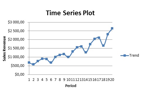
The time series plot above shows the seasonality of revenue and its trend. Seasonality is evident where revenue is low in a certain period and high in another period. These periodic fluctuations are regular. Their cyclical nature is confirmed by the repeated swings over the five years. The time series plot also shows an upward trend i.e. data is increasing over time.
The summary of regression output gives a trend line: Y=92.63X+375.18. (Wang and Chaman 25). This trend line means that sales revenue will change 92.63 times for each increment in period X. The regression output also shows an R square of 0.8726. This implies that 87.26% of the variations in sales revenue are explained by period, x.
Table of seasonal variations seeks to highlight variations that are anticipated in the trend. Looking at the table below, the sales revenue of the first quarter will vary by 111% from the trend line. A similar observation is drawn from Q2, Q3, and Q4. It is expected that the total seasonal variation will be in the region of 400%. A variation from this value is however expected simply because of estimation done in the whole exercise.
Seasonal Variations
To obtain seasonally adjusted forecast, trend estimate is multiplied with seasonal variation. This is tabulated on a table.
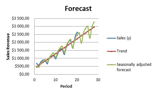
Seasonally adjusted forecast
Forecasts for all quarters during the years 2005 and 2006 have been highlighted. The respective formulas applied in forecasting are available in an excel spreadsheet. Seasonality and trend in projected sales revenue are evident in the table. The highest projected revenue is in the fourth quarter. This observation is also confirmed by the time series plot of the forecast shown below.
It is expected that forecasted sales revenue will differ slightly from actual sales revenue. These differences are explained by random differences. Choosing a regression approach as opposed to a moving average approach also generates errors in forecasting. It is also important to note that people cannot be certain about the future thus predicted values might be different from the actual values. However, the errors can be minimized by choosing the best alternative i.e. with the least errors.
Conclusion
Sales revenue for all quarters in 2005 and 2006 were forecasted using historical sales revenue data for five years starting with 2000. To aid in understanding trend and seasonality, visual diagrams were drawn. The regression approach was mainly deployed in carrying out the forecasts.
Works Cited
Wang, George, and J. Chaman. Regression Analysis: Modeling and Forecasting, New York: Graceway Publishing Company, 2003. Print.