Fiscal Budget Decision and Gross Domestic Product

Introduction

This is a case of a developing economy where the government has a supplemental $2 billion budget meant for policies to boost per capita Gross Domestic Product (GDP) over a 15-year planning horizon.

Two proposals have been tabled. The first aims to raise the literacy, competence, and self-sufficiency of the population by funding an increase of 6 percentage points in the percentage of the secondary school-age population that is enrolled, aiming to reach 61% at the end of fifteen years. But this is a long-term benefit for the population whereas the banking sector of the country is currently in crisis. The ratio of Private Credit by Deposit Money Banks and Other Financial Institutions to GDP has fallen steeply to 0.38 (from 0.52 in the prior period), thus imperiling the liquidity of the system and all business activity dependent on loans from local banks. As this threatens an immediate slowdown in business activity and a consequent reduction in per-capita GDP, the government has been asked to allot emergency loans to the sector. The analytical task, therefore, involves an empirical model to test which alternative is more likely, all other things equal, to raise per-capita GDP.

Data Compilation and Variable Transformation

The compiled data is shown in Table 1.

Table 1: All Required Logged and Calculated Data

First Test of Hypotheses for the Empirical Model

When historical data PCI ch is employed as the dependent variable in a model using the above logged and transformed data, the coefficients derived (Table 2 overleaf) result in the following model:

• dlypc_i = β₁ + β₂lypc90_i + β₃lseced_i + β₄govgdp_i + β₅open_i + β₆infl_i + β₇credit_i + u_i
• dlypc_i = 1.59 – 0.92 (lypc90) + 0.58 (lseced) + 0.26 (govgdp)+ 0.10 (open)+ 0.38 (infl)+ 0.39 (credit)

Table 2: Calculated Coefficients

An ANOVA on the overall model. This represents a test of the:

• Null hypothesis H₀: β2=β3=β4=β5=β6=β7=0
• Alternative hypothesis H1: β_{1 ≠} 0

Table 3 (overleaf) reveals such an elevated F value that it is associated with a significance statistic p < 0.05, suggesting that beta coefficients greater than zero could have resulted by random chance alone just three or four times in a hundred derivations of empirical data. As this meets the minimum hurdle of p = 0.05, one rejects the null hypothesis and accepts the alternative that the independent variables do influence the growth of per-capita income.

Table 3:

Performing single-factor regression runs for all the independent variables, one finds that:

• From a rather low negative value, β₂ for the variable lypc90 improves from -0.915 in the multiple-regression model to -0.036. But the t test results in such a low value of -0.25 that the significance statistic comes to just p = 0.81, clearly no enough to rule out chance occurrence of a relationship between the logged value in 1990 and PCI ch.
• The hypothesis test for this one-to-one regression also implies that log transformation of per-capita GDP in 1990 cannot per se ably predict the growth of the logged value dlypc 1990 to 2005. Table 4 (overleaf) reveals an F value for β₂ so inadequate random occurrence cannot be precluded.

Table 4: Hypothesis Test for β₂

Taking just the variable seced (percentage of those of secondary school age enrolled as of 1990), the outcome is a coefficient that falls to 0.052 from 0.577 in the multiple-regression model. The t-test derived is so marginal (0.35) as to yield an unsatisfactory significance statistic p = 0.73, certainly nowhere near the 0.05 minimum requirement at the 95% confidence level.

The one-to-one hypothesis test (Table 5) is similarly dissatisfying. β₃ bears an F value so marginal that the coefficient might have cropped up one-fourth of the time that a compilation of international macroeconomic data is processed. One must therefore accept the null hypothesis and state that the log of secondary enrolment rate in 1990 cannot, by itself, be used to predict the rise from 1990 to 2005 of the logged value dlypc.

Table 5: Hypothesis Test for Logged SECED

Reducing the required confidence hurdle to 90% CL for the single-IV model employing involving credit (ratio of private credit by deposit money banks and other financial institutions to GDP in 1990), the result is that the for β₇ coefficient falls from 0.390 (multivariate model) to only 0.109. Even worse, the t test calculated for this beta coefficient is so abysmally minimal (0.76) that the significance statistic is p = 0.45. This is tantamount to saying that the stated value of β₇ about every other time, same as coin-toss odds, an analytical model is run. This is the same outcome one gets for the hypothesis test (Table 6): an F value for β₇ of just 0.57 and p = 0.45. We are unable to reject the null hypothesis and must conclude that the ratio of private-sector credit to local GDP in 1990 has no empirical value for “predicting” the rise in logged value dlypc from 1990 to 2005.

Table 6: Hypothesis Test for Ratio of Private-Sector Credit to GDP as of 1990

The Allocation Problem

The base empirical model suggests that ceteris paribus, allotting $2 billion to prop up domestic lending activity impacts per-capita income more favorably.

If one first removes from consideration the credit variable and reformulate the model, and recalculate by inputting average values for the five other independent variables (except for inserting the 61% goal for seced)…

• dlypc_i = β₁ + β₂lypc90_i + β₃lseced_i + β₄govgdp_i + β₅open_i + β₆infl_i + β₇credit_i + u_i
• dlypc_i = 1.01 – 0.515 (lypc90) + 0.408 (lseced) + 0.222 (govgdp)+ 0.044 (open)+ 0.394 (infl)
• dlypc_i = 1.01 – 0.515 (8.49) + 0.408 (0.61) + 0.222 (16.14)+ 0.044 (47.93)+ 0.394 (0.1)

If the $2 billion were allocated to policy measures designed to increase secondary school enrolment rates immediately, the outcome will likely be an average improvement of 2.62% in per-capita GDP on the fifth year and 10.5% in the 15-year planning horizon. One needs to treat this finding with caution, however, since education explains only 8% of the total variance in the per-capita income growth for the typical developing market.

In turn, deciding to allocate the supplemental budget in support of private-sector credit requires replacing seced in the model with credit. Then the outcome is:

• dlypc_i = 0.925 – 0.40 (lypc90) + 0.235 (govgdp)+ 0.12 (open)+ 0.39 (infl) +.33 (credit_i)
• dlypc_i = 0.925 – 0.40 (0.849) + 0.235 (16.14)+ 0.12 (47.93)+ 0.39 (0.1) +.33 (0.405)

The latter model explains rather more (9.4%) of the total variance in per-capita GDP growth. By the end of the 15 years targeted, one has reason to believe that a 2% annual rebound in PCI ch would cumulate to 30.9%.

Diagnostics

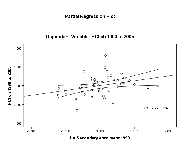
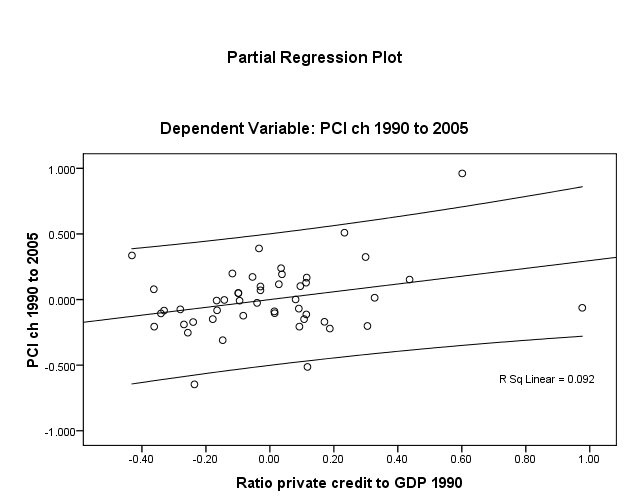
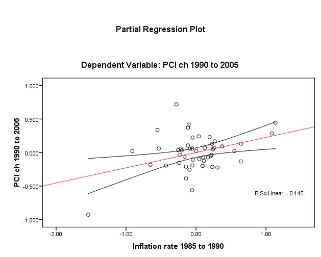
To test the linearity assumption for Y (dlypc_i ), seced and credit, one first has recourse to visual inspection of plots (Figs. 1 and 2, overleaf). These do show a positive linear relationship though unadjusted R₂ ≈ 9% in both cases and there is considerable dispersion around the mean of credit.

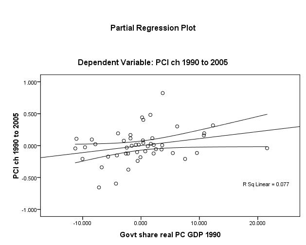
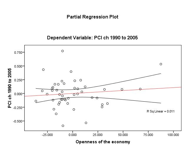
Plotting to check the same assumption for the three other IV’s, Figures 3 to 5 (page 13), reveal that one discerns that openness (unadjusted R₂ ≈ 1%) bears the weakest linear relationship. Nonetheless, the linearity assumption appears to be met for β_i.

The homoscedasticity assumption is essentially met by the fact that all IV’s are either interval or ratio and continuous “scales”. And as long as the use of dummy variables (normally classed nominal or categorical) is limited to the IV’s, the assumption of homoscedasticity holds.