Introduction
The aim of the experiment was to validate Kirchhoff’s Rules as applied in electrical circuits. The practical work was undertaken virtually by using the PhET interactive simulation (PHET Interactive Simulations, 2021). The setup was designed and arranged as shown in the figure below. The lab work employed the general knowledge that distinct methods are utilized to study electronic circuits that are not reducible to simple parallel circuit sequences. The voltage differences and currents across the resistors cannot be examined by applying the general Ohm’s Law. Points D and A are referred to as junctions as at least two wires intersect there.
A closed-loop comprises any path that commences at a particular point in the circuit, flows through the circuit’s elements, and returns to the same initial position. From the figure, the three closed loops are A-B-C-D-A, A-D-E-F-G-A, and B-C-D-E-F-G-A-B. The loops and junctions are employed to study the circuit using the two Kirchhoff’s laws, namely the Kirchhoff’s Current Rule (KCR) and Kirchhoff’s Voltage Rule (KVR). KCR stipulates that the summation of currents flowing into the junction is equal to the sum of currents from the intersection. KVR states that the algebraic sum of the voltage drops within any confined loop is equivalent to zero.
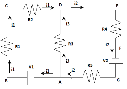
Labeling and arbitrarily assigning current flow directions on every circuit portion, the junction equation at D yields: l1 + l3 – l2 = 0 (I)
Traversing the closed loops in random directions and setting all the voltage changes to zero, the equivalent equation becomes: Σ ΔV = 0 (II)
Where Ohm’s Law gives the voltage difference across the resistance (∆V) expressed as: ΔV = IR (III)
From the preceding expressions, the equations for the three loops can be represented as follows:
Loop A-B-C-D-A with A as the commencing point and assuming clockwise flow: V1 – I1R1 – I1R2 – I3R3 = 0 (IV)
Loop A-D-E-F-G-A with A as the starting point and a clockwise flow: – I3R3 – I2R1 + V2 – I2R5 = 0 (V)
Loop B-C-D-E-F-G-A-B, which is a dependent equation derived from the summation of equations (iv) and (v), yields: + V1 – I1R1 – I1R2 – I2R2 + V2 – I2R5 = 0 (C)
Theoretically, the solutions for the unknown currents ( I1, I2, I3) in the simultaneous equations are achieved by solving equation (I) and two other equations picked from equations (IV), (V), and (V). The negative current attained from computations implies that the current was flowing in the opposite direction from the arbitrarily assigned direction.
Procedure
- Five resistors labeled: R1, R2, R3, R4 ∧ R5, with resistances of 10Ω, 15Ω, 20Ω, 25Ω and 30Ω, respectively, were selected.
- The resistors were arranged and connected on the PhET simulation forming the initially shown circuit diagram. Two batteries of voltages V1 and V2 measuring 7.5V and 9.0V, respectively, were fixed in their designated points of the circuit. The resistors R1, R2, R3, R4 ∧ R5 were also attached to their appropriate positions in the circuit. With the complete setup, the potential differences across the batteries were measured using a voltmeter and recorded as V1 and V2.
- The currents I1, I2, I3 were computed by employing the two Kirchhoff’s Rules and the known battery voltages and resistances. The worked-out currents were used in Ohm’s Law for the calculation of the voltage drops across every resistor. During computation, equivalent current directions and notation were utilized as depicted in the schematic diagram.
- With the theoretical figures’ rough idea, the potential difference across each resistor was afterward measured and recorded.
- The readings of the main currents I1, I2, I3 were then made using an ammeter. This was achieved by snapping the circuit and inserting the ammeter in series with the loop wires.
- Finally, the deviations between the computed and weighted figures of the voltages and currents were calculated, and the percentage errors were derived. Verification of the loop rules and Kirchhoff’s laws was also done.
Data Observations
Measured Voltages V1 and V2
Measured Currents and Voltages across Resistors
Measured Currents I1, I2, I3
I1 = 0.25
I2 = 0.19
I3 = 0.06
Data Analysis/ Calculations
Theoretical Calculation of I1, I2, I3
- From equation (I) l1 = l2 + l3
- Substituting the values of resistors into equation (IV) yields
- 7.5 – 10I1 – 15I1 + 20I3 = 0
- 25I1 – 20I3 = 7.5
- Substituting the resistors’ figures into expression (V) yields
- –20I3 – 25I2 + 9 – 30I2 = 0
- 55I2 + 20I3 = 9
- Replacing I2 in equation (VII) into equation (IX) yields
- 55(I1 + I3) + 20I3 = 9
- 55 I1 + 75I3 = 9
- Solving equations (VIII) and (X) simultaneously yields
- 55(25I1 + 20I3) = 7.5
- 25 (55I1 + 75I3) = 9
- -2975 I3 = 187.5
- I3 = 187.5/-2975 = -0.06 A
- From equation (VIII), I1 = 7.5 + 20I3/ 25 = 7.5 + 20(-0.06)/25 = 6.3/25 = 0.25A
- From equation (VII), I2 = I1 + I3 = 0.25 + (-0.06) = 0.19A
Verifying Kirchhoff’s and Loops Rules
- From I1 + I3 – I2 = 0
- 0.25 + (-0.06) – 0.19 = 0
- 0=0
From loop A-B-C-D-A equation (one of the loops)
- V1 – I1R1 – I1R2 + I3R3 = 0
- 7.5 + 0.25 (10) – 0.25 (15) + (-0.06)(20)
- 7.5 – 2.5 – 3.75 – 1.2 = 0
- 0.05 = 0
- 0=0
Potential Differences across Resistors
Vr1 = I1 x R1 = 0.25 x 10 = 2.50 V
Vr2 = I1 x R2 = 0.25 x 15 = 3.75 V
Vr3 = I3 x R3 = 0.06 x 20 = 1.20 V
Vr4 = I2 x R1 = 0.19 x 25 = 4.75 V
Vr5 = I2 x R5 = 0.19 x 30 = 5.70 V
Data Comparison and Percentage Errors
Conclusion
From the data analysis, it was observed that the computed value of I3, was negative, suggesting that the current flow was counter-clockwise in the assumed direction. The measured and calculated values of currents across individual resistors did not vary since the primary current remained constant. Further, percentage errors between the measured and calculated voltages were minimal due to a lack of active human involvement. Nevertheless, the virtual lab was a success as Kirchhoff’s Rule and loop rule were demonstrated and verified.
Reference
PHET Interactive Simulations (2021). Circuit construction kit: Dc – virtual lab.