About Non-Parametric Procedures
The most common reasons of selecting a non-parametric test over the parametric alternative
Non-parametric tests are preferable over parametric tests in case the data has violated the assumptions of normality (data does not have a normal distribution). Non-parametric tests are also preferable over parametric tests if the data does not maintain the assumption of homogeneity of variances (if the variances are assumed to be unequal). Finally, non-parametric tests are choices where the observations are not guaranteed to be independent (randomly selected) unlike in parametric tests which assume that the observations are made independently (Field, 2009).
The issue of statistical power in non-parametric tests (as compared to their parametric counterparts), and type that tends to be more powerful
In general, parametric tests have a relatively higher statistical power compared to their non-parametric counterparts. For instance, the Friedman test contains a lower statistical power compared to repeated measures ANOVA because the Friedman test has no assumption for normal distribution. This argument prevails in the explanation of lower statistical power in all other non-parametric counterparts of parametric tests.
It is notable that the statistical significance generated in both parametric and non-parametric tests is almost the same. However, non-parametric tests have lower statistical power for detecting differences but this loss of power is reduced as the relationship between the variables becomes stronger. Non-parametric tests have less statistical power because power is usually not straightforward in that it is calculated via simulation methods. This is unlike the calculation of power in parametric tests where formulas and tables graphical displays aid in calculating the power (Field, 2009).
For each of the following parametric tests, identify the appropriate non-parametric counterpart:
Non-Parametric Equivalents of Parametric Tests
A non-parametric version of the dependent t-test (Wilcoxon Test)
Table 1 shows that among the 40 students who did the creativity pre-test, the mean score was 40.15 with a standard deviation of 8.30, while the mean creativity posttest score was 43.35 with a standard deviation of 9.56. Table 2 shows that there were 9 cases where creativity pretest scores were higher than creativity posttest scores and 28 cases where creativity posttest scores were higher than pretest scores. There were three ties indicating that there were three cases where creativity pretest scores were the same as posttest creativity scores. The mean sum of negative ranks is 15.67 whereas the mean sum for positive ranks is 20.07.
It is therefore evident that posttest scores were higher in general compared to pretest scores. Table 3 shows that the Z value is -3.179 and this has a 2-tailed significance value of.001 indicating that the difference between the pretest scores and posttest scores was statistically significant. The Wilcoxon test is based on negative rank in this case since the negative rank contains the smallest sum of ranks (141.0).
I summary, the Wilcoxon test (based on negative ranks) conducted to assess whether creativity posttest scores were significantly higher than pretest scores indicate a significant difference between pretest scores and posttest scores, (Wilcoxon Z = -.3179, p <.05). Since this is based on negative ranks, the significance of this test implies that post-test scores were higher than pre-test scores after the 12 weeks course.
A non-parametric version of the independent t-test (Mann-Whitney U)
The average rank for creativity pre-test scores, N = 40 was 32.66 while the average rank for creativity post-test scores, N = 40 was 44.78 (Table 4). This means that creativity test scores tended to increase with time ranging from the start of the course (Week 0) to the end of the course (Week 12). On applying the Mann-Whitney U test on creativity test scores, it was found that there was no significant difference between pretest and posttest creativity scores, (U = 629.00, p =.10) (Table 5). It is important to note that this finding contradicts the findings of the independent t-test that found that there was a significant difference between creativity pretest and posttest scores. This is an indication that the Mann-Whitney U test (non-parametric) has a lower statistical power compared to the parametric counterpart (independent t-test).
Non-parametric version of the single factor ANOVA (Kruskal-Wallis Test)
The mean systolic blood pressure is 124.77 with a standard deviation of 9.03. The mean diastolic blood pressure is 82.90 with a standard deviation of 2.83 (Table 6). The mean rank for systolic blood pressure taken at home is 14.25 whereas the mean ranks for systolic blood pressures taken at the doctor’s office and in the classroom were 22.80 and 9.45 respectively (Table 7). The mean rank for diastolic blood pressure taken at home setting was 15.75.
The mean ranks for diastolic blood pressures taken at the doctor’s office and in a classroom setting were 16.30 and 14.45 respectively. This indicates that the mean ranks for either type of blood pressure taken at the doctor’s office are higher than when blood pressure is taken in the classroom or at home.
A Kruskal-Wallis test was conducted to evaluate differences between systolic and diastolic blood pressures in three settings (home, at the doctor’s office and in a classroom). There were significant differences in systolic blood pressures in the three settings, Chi-Square (N = 30) = 11.85, p<.05. However, there was no significant differences in diastolic blood pressures in the three settings, Chi-Square (N = 30) =.237, p >.05 (Table 8).
Sometimes a Mann-Whitney U test is conducted to clearly identify where differences in the groups (in this case the three settings occur (Field, 2009)). However in this case, it is clear that systolic blood pressures differ significantly in the doctor’s office than in any other setting. This implies that when blood pressure is measured at the doctor’s office, patients tend to record high systolic blood pressures than when blood pressure is taken in other settings such as home or in a classroom where people are perceive the environment to be normal. This therefore confirms that the participants of this study actually experienced white coat syndrome out of the perception that they are in an abnormal setting.
A non-parametric version of the factorial ANOVA (Friedman Test)
A Friedman test was conducted to evaluate differences in mean of math scores among grade 5 children in classes of different sizes (10 or less children, 11-19 children and 20 or more children). The test was significant, Chi-Square (N = 60) = 60.00, p<.05 (Table 11). The mean rank for classroom size is 1 whereas the mean rank for math score is 2. The significant Friedman test implies that the alternate hypothesis that there is a difference in math scores when children are in classrooms of different sizes to be accepted. The high Chi-Square value is also a clear indicator that classroom size and math score are related variables and their relationship is that an increase or decrease in classroom size causes a significant change in math score attained by children in either gender. One would therefore expect to have different math scores in classes of 10 or less children when compared to classes with 11-19 children or classes with 20 or more children.
Contingency Tables
Table 12 shows that 927 (65.3%) of a total 1419 cases were used to generate a contingency table between education (degree) and perception of life (life). Table 13 shows the observed and expected counts and frequencies for different life experiences (exciting, routine and dull) in relation to level of education (less than high school, high school level and junior college education). The observed count for persons’ with an education less than high school and who view life as exciting is 52 (50.8%) while the expected count is 77.0.
For individuals with less than high school education and who have the perception that life is dull, there is an observed count of 95 (21.3%) and an expected count of 79.1. Still in the group of individuals with less than high school education, there is an observed count of 17 and an expected count of 8.0 of persons who view life as dull.
For individuals with a high school education, there is an observed count of 221 (50.8%) and an expected count of 226.7 individuals who had a perception that life is exciting. There was an observed count of 242 (54.1%) and an expected frequency of 232.9 of person with a high school education and whose perception of life is that life is just a routine. Of the 483 individuals who had a high school education, there was an observed count of 20 (44.4%) individuals and an expected count of 23.4 persons who were of the view that life is dull.
Among the 280 participants who had a junior college education, there was an observed count of 162 (37.2%) persons and an expected frequency of 131.4 persons who viewed life as being exciting. An observed count of 110 (24.6%) and an expected count of 135.0 of individuals with a junior college education perceived life to be a routine. For those who viewed life to be dull and had a junior college education, there was an observed frequency of 8 (17.8%) and an expected frequency of 13.8.
From Table 14, there is no cell that has less than a count of 5. The Pearson Chi-Square value is 36.63 and it has 4 degrees of freedom and its 2-tailed probability is.001. (Pearson Chi-Square = 36.63, df = 4, p =.001). This means that there are significant differences in life experiences among persons with different levels of education (less than high school, high school level and junior college education).
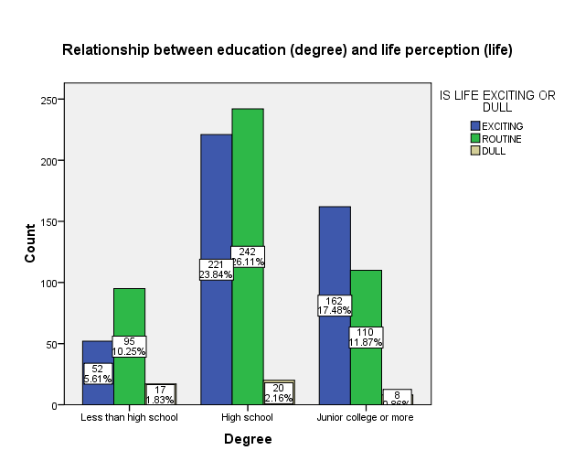
The differences in life perception according to level of education have also been displayed graphically as shown in Figure 1. The findings displayed in Figure 1 affirms the results displayed in the 2 by 2 contingency table thus adding more weight to the hypothesis that education and perception of life are dependent. Figure 1 shows that 52 (5.61%) of participants who had less than high school education felt that life is exciting as compared to 221 (23.84%) of participants who had a high school education and 162 (17.48%) who had a reached at least junior college level of education. 95 (10.25%) of individuals who had less than high school education expressed that life is routine compared to 242 (26.11%) of those who had a high school education and 110 (11.87%) of individuals with at least a junior college level of education.
Figure 1 also shows that 17 (1.83%) of individuals who had less than high school education felt that life is dull compared to 20 (2.16%) of individuals with a high school education and 8 (0.86%) of those who had at least junior college level of education.
In summary, there are more high school degree holders with a perception of life as exciting followed by individuals with at least junior college education. Individuals with less than high school education have the least perception of life as exciting. In the same pattern, the highest numbers of individuals who perceive life to be routine have a high school education followed by junior college individuals. The lowest number of individuals with a view of life as routine belongs to the persons with less than high school education. The least number of individuals with a perception of life as being dull have at least junior college education, while the highest number of individuals who view life as dull have a high school education.
Since the Chi-square test is statistically significant (Chi-Square = 36.63, 2-tailed p =.001), it is evident that there are differences in the way people view life when one considers the level of education. The contingency table (Table 13) actually shows that there are differences between the observed counts and the expected counts of life perception in all the education levels. This is a clear indicator that education level and life perception are related/dependent. Furthermore, the Chi-Square value is very large. The minimum expected count for the Chi-Square test is 7.96. It is on this basis that the null hypothesis (education and perception of life are independent) is rejected and instead the alternate hypothesis (education and perception of life are dependent) is accepted.
On paying closer attention to the contingency table (Table 13), it is evident that the smallest differences in observed and expected counts are found in the high school individuals in all the three life perception categories (5.7, 10.9 and 3.4 in for exciting, routine and dull life perception respectively). The differences in observed and expected counts on perceptions of life increase for those with at least junior college education (30.6, 25 and 5.6 for exciting, routine and dull perception of life respectively). Relatively high differences in expected and observed counts also appear in those who have less than high school education (25, 15.9 and 9 respectively for exciting, routine and dull life perceptions respectively).
It is the large differences in expected and observed counts in all categories of education that result into a big Chi-Square value indicating relatedness of education and life perception. This can only be slightly ruled out for high school education individuals since the differences are relatively small. However, the overall conclusion is that perception of life and education are related and thus the null hypothesis is rejected.
Reference
Field, A. (2009). Discovering statistics using SPSS (3rd ed.). Los Angeles: Sage. Web.
Appendix
Table 1: Descriptive Statistics for Creativity Pretest and Posttest Scores.
Table 2: Wilcoxon Signed Ranks for Creativity Pretest and Posttest Scores.
Table 3: Wilcoxon Signed Ranks Test for Creativity Posttest and Pretest Scores.
Table 4: Mann-Whitney Ranks for Creativity Posttest and Pretest Scores.
Table 5: Mann-Whitney U Test for Creativity Pretest and Posttest Scores.
Table 6: Descriptive Statistics for Diastolic and Systolic Blood Pressure.
Table 7: Kruskal-Wallis Ranks for Systolic and Diastolic Blood Pressures in Different Settings (Home, Doctor’s Office, and Classroom).
Table 8: Kruskal-Wallis Test for Systolic and Diastolic Blood Pressures in Three Settings (Home, Doctor’s Office, and Classroom).
Table 9: Descriptive Statistics for Math Score in Different Classroom Sizes (10 or less children, 11-19 children and 20 or more children).
Table 10: Friedman Ranks for Math Score in Different Classroom Sizes (10 or less children, 11-19 children and 20 or more children).
Table 11: Friedman Test for Math Score in Different Classroom Sizes (10 or less children, 11-19 children and 20 or more children).
Table 12: Number of Cases Processed for Degree*Is life Exciting or Dull.
Table 13: A Contingency Table for Degree*Life Experience.
Table 14: Chi-Square Tests for Education*Life Experience.