Normative vs. Positive Analysis
Economics, at large, belongs to the sphere of academia. Still, economists often perform consulting, analytic, advisory, and other roles. Consequently, it is critical that an economist is skillful at making statements and judgments on the function of government policies and can evaluate them to determine the most optimal tools and business practices.
Normative and Positive analyses can, therefore, be defined as analytic perspectives of economics expressing their assumptions on the objectives and outcomes of government policies. Many sources refer to them as “normative economics” and “positive economics.” Normative analysis can be characterized by its subjectivity and the fact that it bases every assumption on values. In contrast to normative, positive analysis is distinguished by its objectivity; facts are what it bases its statements on.
In its statements, normative analysis operates with imperatives: should, ought, must, etc. A statement made from a normative perspective can be formed as follows: “The government must cut back on taxes to increase the after-tax returns.” This statement can be classified as normative because it is consistent with judgments of values. As a consequence, normative analysis is often dubbed “what ought to be.”
Contrastingly to normative, positive economics is aimed at describing and explaining the existing phenomena. It uses factual evidence of the current processes and relies on the experience of the past to explain and predict the possible outcomes in the future. Given the objectivity of such analysis, its empirical value can be tested as to its truthfulness. A positive statement can be formulated as follows: “The increase of the interest rates will foster long-term saving” or “The unemployment rate has shown a 9% decrease in 2016 compared to 2015.” Because it is evidence-based and refrains from subjective judgment, it is most concisely described as the analysis of “what is.”
It appears that positive economics should prevail because of its objectivity. However, many economists have difficulties confining themselves to rendering sole facts. To make a statement about government policy, one should combine the arguable factual evidence and the subjective value component. The implication of such combination can result in statements that both state the most desirable outcomes (the normative component) and the most optimal means of achieving it (the positive component). As a result, the best part of the information rendered in the mass and social media is a compilation of these two approaches to economic analysis.
Hotelling’s Linear City Model
The model in question was devised by Harold Hotelling in his work “Stability in Competition,” first published in 1929. The model developed the notion of territorial balance within a duopoly where two establishments have to demarcate the territories they take up, about the localization of consumers and prices for transportation. The firms, therefore, have to consider three factors: the competitor’s territorial position, the distribution of customers, and the prices. These variables are supposed to help the firms to choose the best location to gain in revenue.
There are two approaches to the Linear City model. The static model implies that the two establishments choose the place and set their prices at the same time. The dynamic model presupposes them to set the prices after having determined the location. The model has received its name because it is best explained using a hypothetical city consisting of one long street; still more comprehensively, one can think of a long beach with two ice-cream street vendors deciding on where to put their stalls.
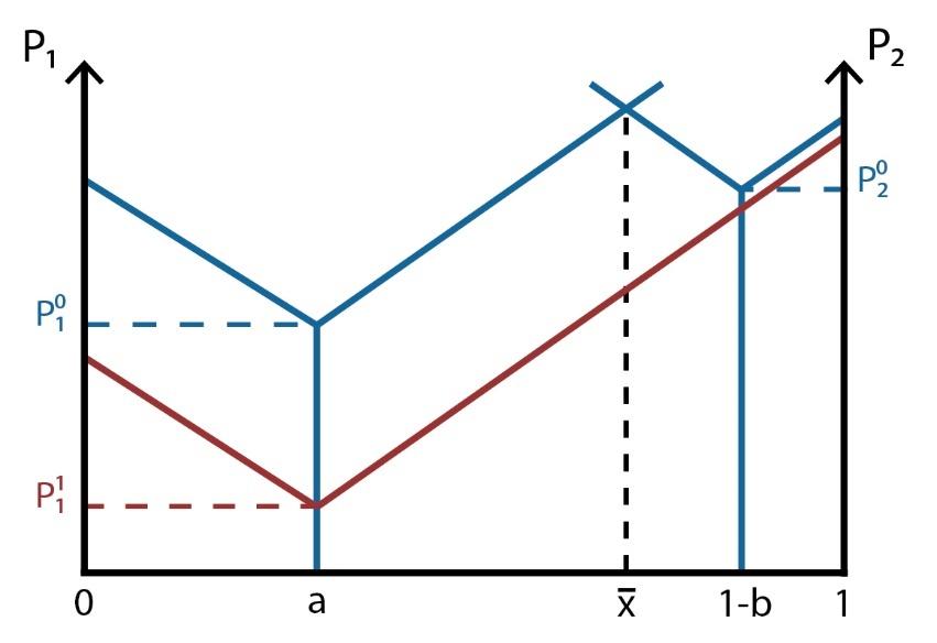
The Static model can be illustrated as follows. Given that the vendors have the same amount of equal quality products, the customers will rely on the distance to each vendor and the price. If the prices are equal, the only variable will be the distance.

If x̄ is the middle of the beach, the customers will either choose stall A or B. For the maximum profits, two conditions are obligatory:
- Marginal costs must be lower than selling costs;
- a ≠ 1 – b or a + b ≠ 1.
The first condition means that the stall with lower marginal cost would decrease the selling ones to push the competitor out of the market. The second one means the stalls cannot be put in the x̄ location because the customers would choose either one of them. Consequently, the vendors would go into damping each other and lose positive profits. As a result, the stalls set their selling costs and choose locations other than x̄.
The Dynamic model features two stages. On Stage 1, the vendors decide on the location. The less distance there is to the extreme, the higher the profits; as a result, stall A can be located at 0 and stall B – on 1, as demonstrated on the graph. Stage 2 is when the stalls set their prices to result in the highest positive profits. Similarly to the Static model, the vendors will set their costs.

The Linear City model is applied in reality by businesses struggling to differentiate themselves firstly by their location and selling prices, which marks the significance of the model to public policy.