The Spannerman Press and Leaflet Campaign: An Evaluation

Executive Summary

Key Findings

On the whole, the plumbing-services chain has shown a preference for allocating more of the local-media advertising budget to leaflets rather than to press advertising. This may seem correct since leaflets are more likely to be kept and contact information therefore easier to retrieve when the need arises. A closer analysis reveals, however, that branch revenues have more to do with the level of effort in local newspapers and periodicals.

Recommendation

The 53% share of local ad budgets currently allocated to leaflets promises to be more cost-effective if diverted entirely to local press advertising. After all, raising trade name awareness in this ad channel will make the chain top-of-mind when a plumbing emergency is at hand. From that consumer state of mind, it is easy enough to look up the contact number in phone books or online.

Technical Appendix

Patterns of Spending

Based on the completed annual campaign in 45 city-markets, on the whole, Spannerman is rather more inclined to spend on leaflets than on press adverts. This is based, first of all, on gross expenditure, on range and central locations measures (Table 1 below).

Table 1:

The nationwide breakdown by medium used last year shows that slightly more than half (53%) of local advertising monies was spent on leaflets and the balance of 47% on press inserts. This overall bias towards leaflets seemed confirmed by the measures of location:

• Mean spending for leaflets amounted to £6,613, about 12% higher than average spend for press adverts;
• Though the distribution of community media spend is skewed towards the low end (“right” or “positive” skew), as evidenced by medians that are lower than the means for both types of media, the overall relationship holds true. The midpoint of the leaflet spending distribution curve (£6,593) is about 14% greater than the equivalent point for press advertising. In turn, the starting point (minimum spend) and ending point (maximum) for the leaflet expenditure distribution curve are both higher, by 28% and 13% respectively, than the corresponding range points for local newspaper and magazine inserts.

Boxplots (see Figure 1 below) provide another way of quickly grasping measures of both central location and dispersion. This shows, first of all, that the range for leaflet advertising spend is higher, approaching £1,000 at the upper end and definitely higher than the £2913 minimum spend for local press.

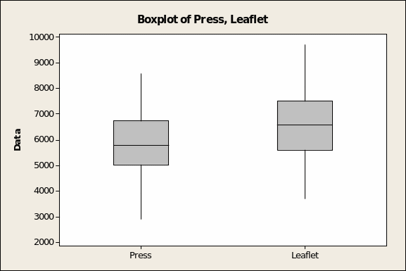
Despite an overlap, the gray boxes that represent the boundaries of the first to the third quartiles range higher for leaflets. And the horizontal line bisecting both boxes, representing the median of each distribution, is also higher for leaflets.

On the other hand, the two measures of dispersion in the Minitab summary table of descriptive measures (Table 1 above) give us pause about the consistency of the spending patterns for leaflets. The standard error of the mean is larger for leaflet spend than for monies allotted to press, which suggests that the associated means are from unequally distributed population means. Even more explicitly, the standard deviation reveals that the dispersion of spending for leaflet advertising is greater.

Table 2: Markets Where Leaflet Spend was Lower

A significant reason for the wider standard deviation is that the overall propensity for leaflets does not apply to all cities where Spannerman does business. Table 2 (alongside) reveals that press spending exceeds that for leaflets in 17 of the markets (38% of the total). So the overall preference for one advertising medium does not hold. Or at least, some other factor influences the mix of local media employed.

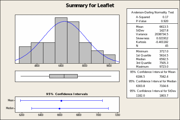
The graphical summary for leaflet advertising (Figure 2 below) affirms little more than that there is a wide dispersion of spending allocations for this medium across all 45 markets. At the same time, it approximates a normal curve.

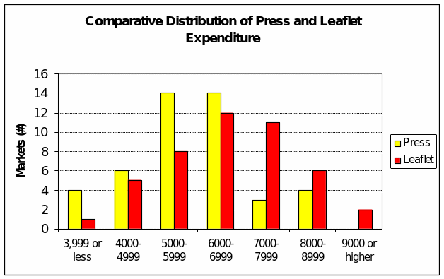
A side-by-side comparison of spending by medium (Figure 3 overleaf) does show that ad spending on leaflets tends to be higher than for mass-circulation city newspapers. However, as we have seen in Table 2, there are exceptions aplenty where just the opposite holds true.

Testing for Significance of Differences

At this stage of analysis, we ask the question, “Is the difference in average spending by medium meaningful or not?” In other words, is the observed difference of 12% in mean expenditure shown in Table 1 meaningful or insubstantial? One way to answer this question is to employ Student’s t test for the significance of differences between means of two related or independent groups.

Understanding the result of the test rests on articulating a null hypothesis: “There is no difference in mean spending for press adverts or leaflets.”

Table 3:

The salient findings of the t test (Table 3 above) start with the absolute difference between the two means, a gap of £ 709 on average between press and leaflet spending levels. If the null hypothesis were true, the difference should be zero or some insignificant value.

Taking into account the “real world” dispersion of the data, the test yields a t value of 2.41. At 87 degrees of freedom, such a t value is associated with a significance statistic p < 0.02 (rounded off from p = 0.018). Since p in this case meets the ordinary threshold of α = 0.05 applicable to most statistical test processes, one interprets the result as saying that the observed difference of £ 709 could have occurred by chance alone less than twice in a hundred “sampling runs” of real world data. Accordingly, one rejects the null hypothesis and accepts the alternative hypothesis: there is a difference in spending propensity by advertising medium.

The Relationship with Branch Revenues

As managerial decisions go, there is usually a correspondence between advertising effort and sales. Theoretically and all other things equal, higher advertising investments should result in improved sales. In practice, it is more often true that subordinate and city/branch business managers plan advertising outlays based on sales growth or decline in preceding periods. Either way, a correlation analysis should reveal some logical relationship between advertising effort (measured as X pounds spent) and revenue outcomes.

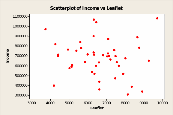
Prior to running correlation and regression analyses on data, it helps to plot the relationships among all three variables. For didactic purposes, we assume that branch income is the dependent variable and spending on the two ad media the independent variables. Figure 4 below shows a random relationship between income and spending on leaflet advertising. On the other hand, Figure 5 (overleaf) demonstrates a positive and linear relationship between branch income and ad spend in local press vehicles.

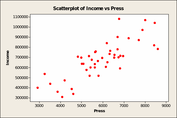
A simple linear regression is appropriate for testing the relationship between income as the IV and level of press advertising as the DV because we at least know from Figure 5 (above) that the two bear a linear relationship.

In table 4 below, the key results of the regression function show that from a baseline annual revenue of about £ 39762, income should increase by £108.40 for every pound spent on local press inserts. The R² value shows that this single independent variable of press advertising explains nearly two-thirds of the variation in sales.

Table 4:

The line of best fit for this relationship is depicted in Figure 6 below. Besides enabling a fairly confident prediction of what revenue results might obtain if more aggressive press placements were the norm, the angle of the line itself suggests that this single medium bears a strong linear influence on sales, all other variables equal, of course.

For the relationship between revenue and leaflet expenditures, on the other hand, the beta coefficient is negative (Table 5, page 11). Theoretically, this means that income should decline by £13.37 for every pound allocated to leafleting campaigns. This is at best an inconclusive result since R² is extremely low and the fitted trend line (Figure 7 overleaf) must be viewed against the extreme scatter of the data itself. We are as close to a flat, entirely random and no-relationship line as “real-world” data can make it.

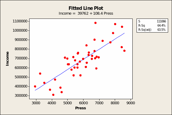
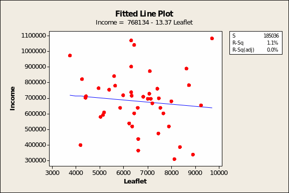
Table 5:

Hypothesis Test for the Regression

This is stated as a null hypothesis such that the slope will be other than zero if there is truly a linear relationship between the independent variable press spending and the dependent variable branch revenue:

• H₀: Β₁ = 0
• H_a: Β₁ ≠ 0

Since, as shown in Table 6 below, the value of P associated with the slope of the regression line for “Press spending” at 44 degrees of freedom is lower than the normal benchmark of α = 0.05, we cannot accept the null hypothesis that this result is due to chance alone. Hence, we accept the alternative that the regression line for this independent variable is positive. There is a relationship.

Table 6: