Introduction
This report proposes to investigate the best ideas that should be considered when taking insurance cover. Also, in this report, the data used for the analysis is from Post Assignment-Insurance Regression. The analysis tool used for data analysis is the R-programming package. The report will be based majorly on the finding from one of the statistical models, Regression analysis(simple Linear and Multiple Regression). Thereafter, there will be a recommendation and conclusion based on the outputs of the analyzed data.
Statistical Terminologies Used
- Calculated Probability Value (P-value) this is the calculated probability value of accepting the generated model, intercepts, and coefficients.
- R2 – the statistical measure of closeness of that on the fitted Regression Line.
- Significant- relevancy of the model of coefficient.
Executive Summary
When taking health insurance coverage, the insurance company needs to optimize both services rendered and profit gained; based on the data from Health Care Annual Expenditure, the statistical model (Regression) will analyze the factors that have a significant impact on the amount individuals spend on health care coverage. Furthermore, the regression model will also filter out “noise” variable that does not add any value but are captured. According to Schmidt and Finan (2018), regarding linear regression and its application to economics, the regression analysis model is preferred as it gives simple and easier interpretable results.
The focus is to find the variable that best predicts the amount one should pay the health care facility in a year. In this case, the dependent variable is the amount paid and other variables will be assumed to be independent.
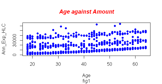
Based on the data from figure 1 above, we can easily conclude that the health care annual expenditure data, age, and amount paid annually can fit a regression line; data is distributed linearly. Therefore age can be the best predictor of the amount a person should contribute towards healthcare coverage.
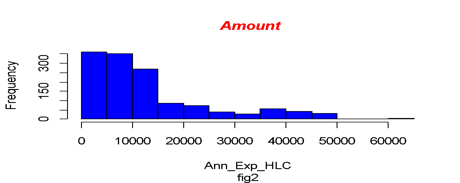
In the above histogram, we can conclude the amount distributed through the data is positively skewed. And to confirm our suspicions, we will find the correlation between Age and the Annual amount paid. Correlation is the statistical term that describes the extent to which two variables are related. There is a positive correlation between Age and the Annual Amount paid to health care of 0.2997677. According to the output, the Coefficient of the simple linear regression is 3138.33 and 258.28 on the intercept and the gradient, respectively. The calculated probability value (p-value) is 2.2e-16. This is compared to the standard Prbobality value for accepting the model of 0.05. the analysis report here shows that the model generated can be adopted.
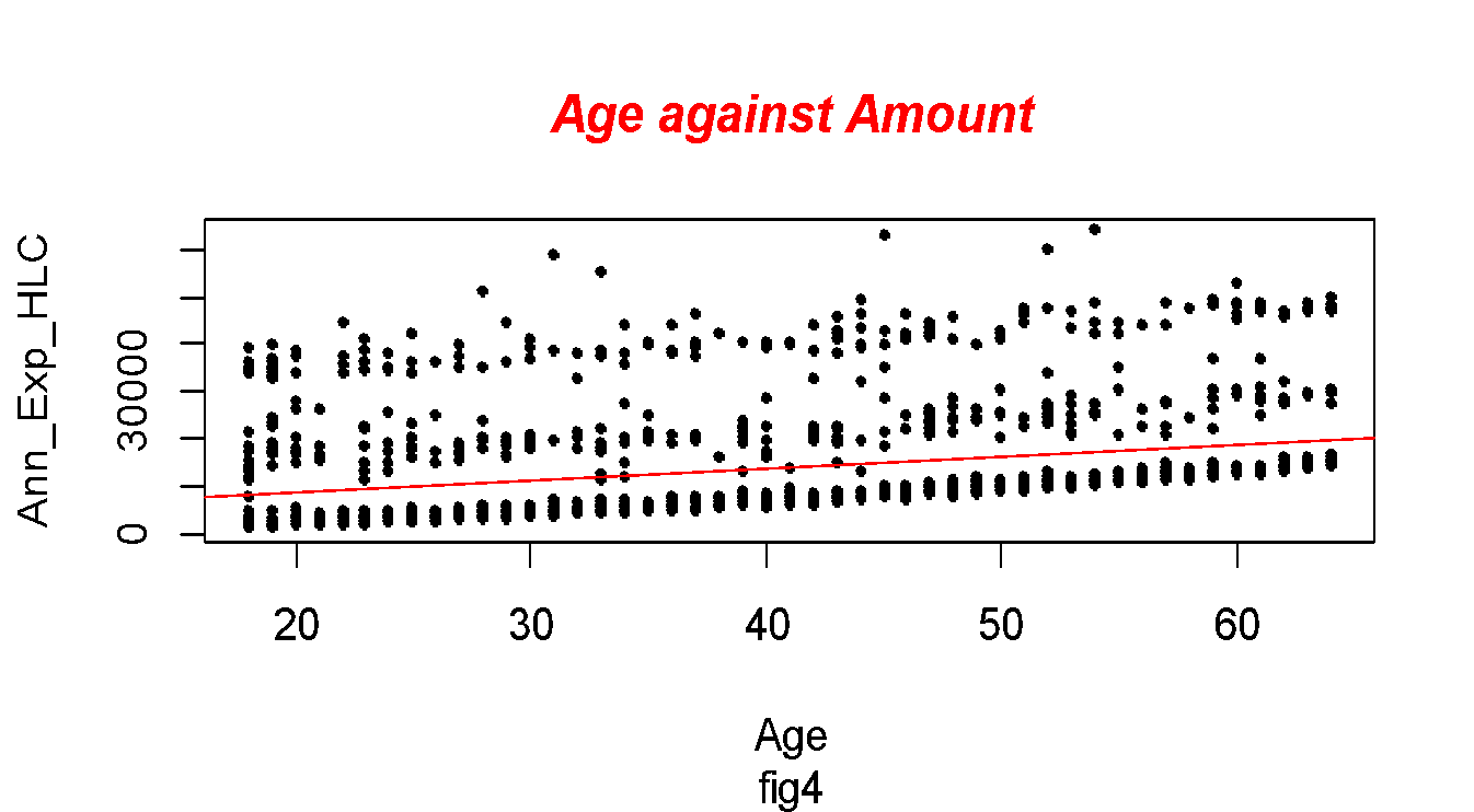
However, (R-Squared) the coefficient of determination on how close the data are to the fitted regression line is 0.089. This implies the model only explained 8.9% of the data, see fig4 below. Further, more, according to Tirgil et al. (2018) it is quite obvious in some areas to get the lower coefficient of determination as some behaviors are hard to predict. The calculated model is shown below;
Y=3138.3253+258.2807 Age, where: Y = Annual Expenditure in Health Care
Simple Linear Regression (Age and Number of Children as Predictors)
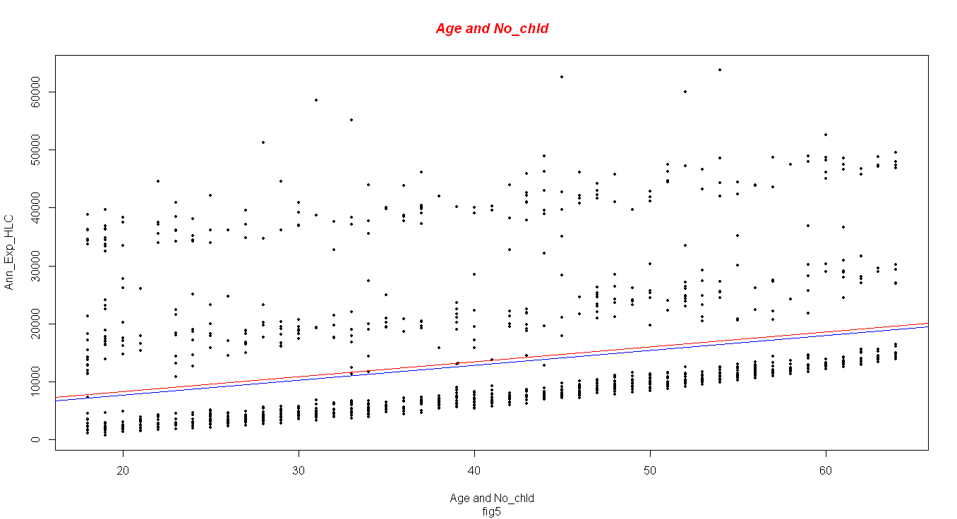
Here, we are going to formulate a regression model that depends on two variables, Age and Number of children. We are interested to see if this variable can give the best prediction on the Annual amount spent (Miot, 2018). The analysis gives a positive correlation between the number of children and Annual expenditure of 0.06863, and the model analysis results are as follows;
The coefficients of the model are 2607.2, 256.2, and 559.8 for the intercept, for Age as an independent variable, and the number of children as an independent variable respectively.
The model follows the following equation;
Y=2607.2+258.2807 Age + 559.8 No.Chld, where Y=Annual Expenditure in Health Care
The general Calculated Probability value of the model is 2.2e-16, this signifies that the model is significant as it is way less than the standard value of 0.05. The coefficient of determination on this second model is 0.09296. As explained earlier, the model explains only 9.3% of the fitted data. Figure 5 gives a visual of how close data is fitted on the regression line.
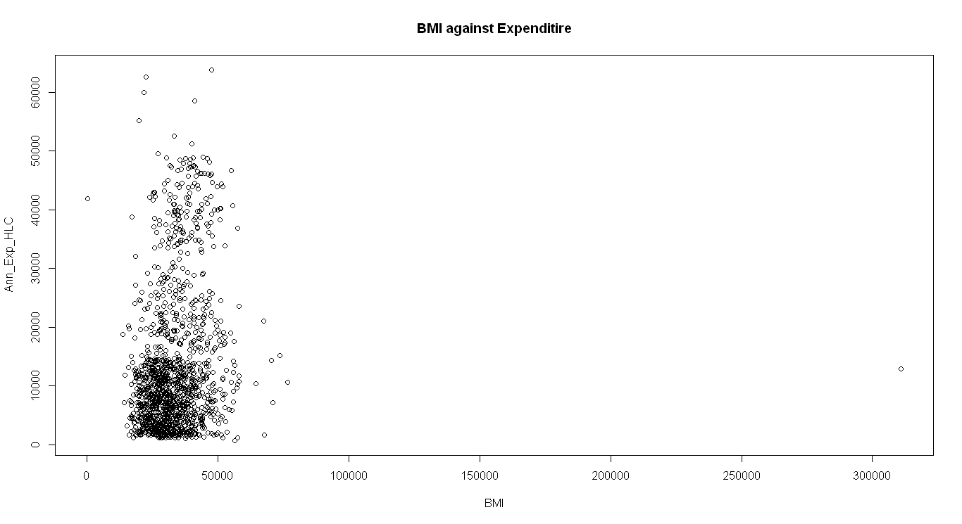
Simple Linear Regression (BMI and Age as Predictors)
In this section, both Weight and Height are interrelated to create a new variable, BMI. Thereafter, analysis is conducted to identify the connection between BMI and annual expenditure. Subsequently, we will try to model and see if the model will signs it will follow a non-linear relationship (Fong et al., 2017). From the model, there is a positive correlation of 0.1655. This infers that BMI and Annual Expenditure are 16.55% related, which means that the weight and height of individuals are less significant in determining the amount to be spent on healthcare.
On running the model in the R-programming package, the model results are as follows;
The general Probability value of accepting the model does not change and remains 2.2e-16; we also need to adopt the new model. However, the model coefficients change significantly as the intercept of the model is -2583.7080, and the coefficients of the other variables are 251.8186, 593.1699, 0.1608 for Age, Number of children (No_ Chld) and BMI respectively the model is
Y=-2583.7080+251.8186 Age + 593.1699 No.Chld + 0.1608 BMI
Moreover, the coefficient of determination in this quadratic relationship is 0.1178. this implies that the generated quadra regression explains 11.78% of the data. BMI does not explain health Care Expenditure according to this analysis and BMI has a unique non-linear relationship, as shown in the figure below. The model explanatory power of the generated model is 12% percent. This is due to several factors that were left out and also, predicting Human behavior is not that easy.
The pictured U-shaped relationship between BMI and Expenditure is caused by the distribution of vulnerable age group that is affected most by diseases.
BMI is not a good explainer of the Expenditure, the weight, and height of a person do not dictate how frequently one will need health attention. Also, gender as one of the recorded variables does not give a clear cut if it should be a determinant of one’s health. Smoking though is left out of the analysis, has a great impact on a person’s health. As smoking will catalyze some the diseases like liver cancer, heart disease, and also infection in the breathing system of a person.
Variables to be Considered in the Model
Alcoholic Status
The other variable that should be considered when someone is taking Health Insurance Cover is alcoholic status; just like smoking, drinking too much has a great impact on someone’s health; it can health emergencies when a person is drunk is very vulnerable to all kind of health attacks.
Employment Status
Further, an additional variable to be considered is the employment status of a person. It is very unfair for the insurance company to approach an employed individual to take insurance coverage.
Effect on the Model
If these new two variables were included in the model, the model would be 90% efficient in explaining the data. Employment status plays a key role in influencing the individual income, therefore, impacting the need to feel secure. The best way of collecting data on these two variables is by examining the government database for civil workers and taking records of employed drinkers.
Limitations
The model does not explain how the gender of a person affects the analysis. Age is not well categorized in this model, should be splitted into sections of young, teen an adults, there are chances of high health instability at young age and adults. A possible wrongful conclusion arising from this model is BMI, the analysis does not give a clear relationship on how it affects the individual’s annual expenditure on healthcare. A different study having the mentioned missing variables or classification can be conducted to verify the relationship between the predictors and the dependent variable.
Recommendations
First, the insurance company to consider key elements when registering one under this cover and set optimum requirements for one to qualify to be insured, this should include the employment status of a person before. Additionally, it ought to consider a person’s family (number of children) or the population an individual wants to cover. These two variables, together with age are key variables to the future models and also increase the efficiency of the model. Secondly, the insurance firm should ensure they formulate premiums to be paid based on the number of children an individual has and the age of the people to be covered. From the analysis, there is a strong correlation between annual expenditure and the people’s age and a total number of kids (Chen & Xu, 2020). Therefore, to be able to protect all the persons, the contribution should be based on the factors. Thirdly, the insurance company should use the health officer to encourage individuals to take health insurance coverage. This initiative will save lives during emergencies since individuals will have protection from the company. Moreover, the government should put directions that all employed civil workers be under health coverage.
Conclusion
Based on the analysis age and number of children is the best predictions of Health Expenditure. These variables are very basic when one wants to take health insurance coverage. The region does not have any impact on the Annual Health Expenditure; although it should be considered during data capturing, it does not determine the Health anomalies of persons. In addition, the suggested variables should be added to the future model as they could increase the explanatory by a higher percentage.
References
Chen, L., & Xu, X. (2020). Effect evaluation of the long-term care insurance (LTCI) system on the Health Care of the Elderly: a review. Journal of Multidisciplinary Healthcare, 13, 863.
Fong, Y., Huang, Y., Gilbert, P. B., & Permar, S. R. (2017). chngpt: threshold regression model estimation and inference. BMC Bioinformatics, 18(1), 1-7.
Miot, H. A. (2018). Correlation analysis in clinical and experimental studies.
Schmidt, A. F., & Finan, C. (2018). Linear regression and the normality assumption. Journal of Clinical Epidemiology, 98, 146-151.
Tirgil, A., Gurol-Urganci, I., & Atun, R. (2018). Early experience of universal health coverage in Turkey on access to health services for the poor: regression kink design analysis. Journal of Global Health, 8(2).