Executive Summary
The analysis of sales data of five products (1-5) offers important information regarding their structure, appropriate models of the forecast, and prediction of demand. The attributes of product 1 indicated that it has a cyclical structure without seasonality and trend. Based on these attributes, SMA and SES were suitable models of forecasting. Product 2 exhibited sales with an additive trend but without seasonality, making the Naïve and Holt’s methods as appropriate forecasting models. In the analysis of product 3, both seasonality and trend were evident. In this view, TSEM and regression analysis fitted in the prediction of sales. Product 4 exhibited seasonality without trend, making SEM and linear regression analysis appropriate models of forecasting them. In products 1-4, MAE and MAPE were suitable in the measurement of errors for accurate forecasting. Product 5 had an intermittent structure of sales, which suited the use of SBA and Croston’s methods. The scaled MSE fitted the measurement of errors in product 5 sales data owing to the sporadic nature of trends.
Introduction
Analysis of sales data is critical in business because it generates information that informs operations and trends of consumer demand. The purpose of this report is to analyze sales data of five products (P1 to P5) and generate forecasts based on time and temperature. To highlight trends in sales data, the analysis decomposed the time series of each product. Further, the analysis employed a feasible candidate method in examining the structures of different sales data. After separating out-of-sample and in-sample datasets, the forecast was done by employing the in-sample one in predicting the trend of sales and creating a reliable model. Subsequently, error measures were selected based on key performance attributes and then employed in the evaluation of the created model. The evaluation of forecast methods and respective error metrics was done to achieve comprehensive findings. Critical examination of findings led to the generation of practical recommendations and conclusions for the company to implement.
Description and Analysis
Time series graphs were plotted for products 1 to 5, depending on frequencies of 100 observations of sales recorded daily and weekly. By examining trends and seasonality, the structure of sales of each product was established. Decomposition was performed to highlight the presence of trends, seasons, and noise attributes of sales.
Product 1
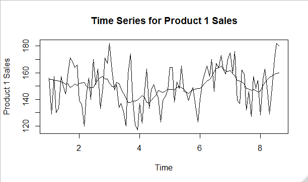
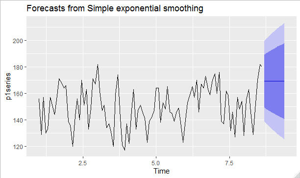
Since the sales of product 1 were collected weekly 100 times, a frequency of 13 was considered appropriate to provide a quarterly times series. The plot also shows a 13-weeks centered moving average (13-CMA) without a clear trend. Figure 1 shows that product 1 exhibits some seasonality because sales appear low in every even quarter and high in every odd quarter.
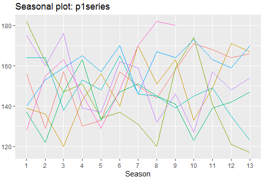
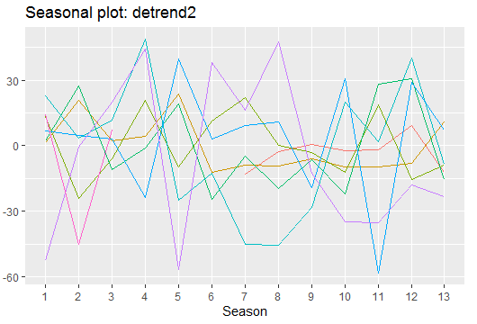
The plot of seasonality (Figure 2) shows that sales of product 1 do not have seasonal variation since the trend lines appear random. The WO-test confirms that the trend of product 1 sales does not have seasonality.
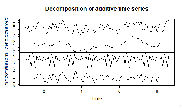
The decomposition of data (Figure3) indicates an irregular structure of product 1 sales and a considerable degree of noise.
Product 2
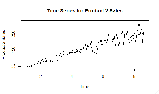
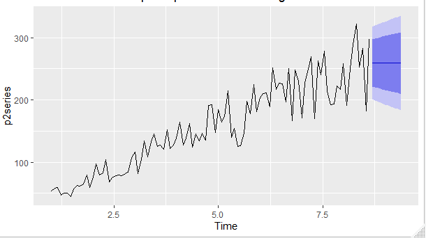
also shows weekly sales recorded over 100 weeks and a frequency of 13 was used for the quarterly analysis of its trend. The sales data shows an increasing trend as shown in figure 4.
The de-trended seasonality plot (Figure 5) shows that sales of product 2 do not exhibit a seasonality trend because it has a lot of noise in the data.
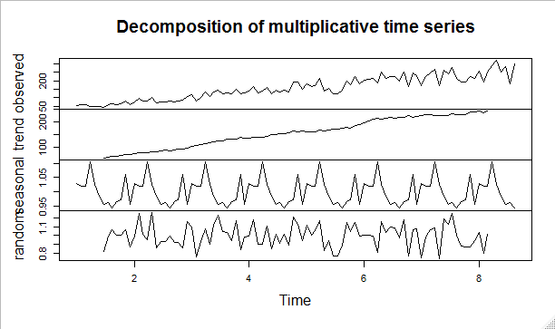
The multiplicative decomposition (Figure 6) depicts that the product has an increasing trend without seasonality. The observed trend seems to be stable up to the fourth quarter where it starts to exhibit significant variability and decline after the seventh quarter. The WO-test confirms that sales of product 2 do not exhibit seasonality in its multiplicative trend.
Product 3
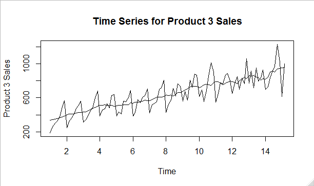
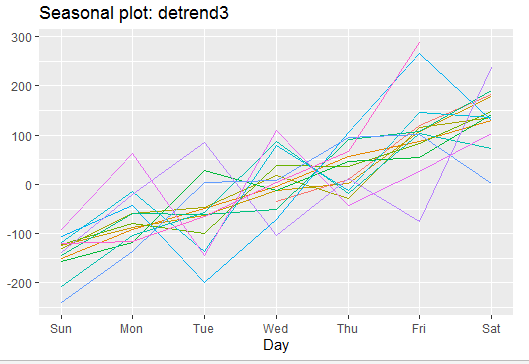
As product 3 sales were recorded daily for 100 days, the frequency of seven was used to analyze the weekly trend of data. Figure 7 shows that sales of product 3 have both additive trend and seasonality with a weekly centered moving average (7-CMA). The de-trended plot shows that sales of product 3 follow the weekly season with a minimal level of noise (Figure 8). The additive decomposition plot shows that product 3 has an increasing trend with a clear pattern of seasonality (Figure 9). The WO-test confirms that the apparent weak seasonality is statistically significant (p<0.001).
Product 4
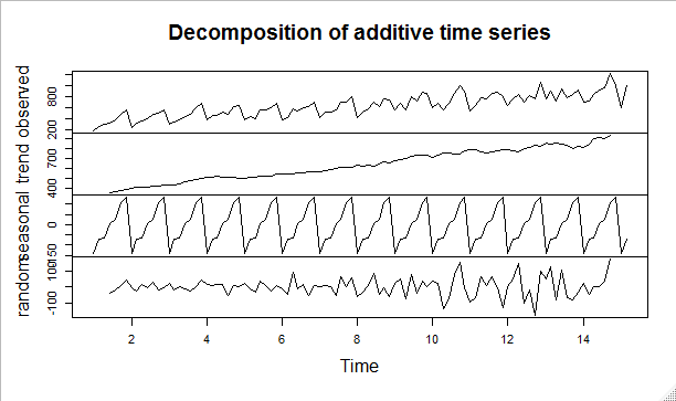
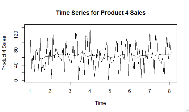
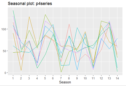
As sales of product 4 were measured daily and weekly trend exhibited a lot of noise, the frequency of 14 days was used (14-CMA). The plot (Figure 10) shows that product 4 sales data do not have a trend since the variation is constant along the trend line. However, the seasonality plot (Figure 11) reveals that sales of product 4 exhibit a fortnightly season with a limited degree of noise. The additive time series (Figure 12) indicates seasonality and an increasing trend in product 4 sales. The WO-test reveals that product 4 sales data has statistically significant seasonality (p<0.001).

Product 5
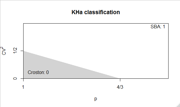
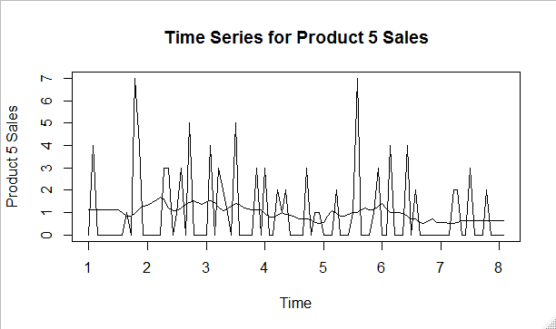
The examination of the plot of product 5 sales shows that it has neither season nor trend, which defines the structure of time series (Figure 13). The existence of zero implies that product 5 has an erratic demand that is hard to predict using standard decomposition methods. Based on the average demand of 0.95 and the squared coefficient of variation, the SBA method indicated that the demand interval was greater than 1.33 (Figure 14). In this view, the SBA model became an appropriate one in forecasting sales of product 5.

Candidate Forecasting Methods
Product 1
Given that the time series plot of product 1 did not have a trend or season with a lot of noise, a linear forecast method is suitable. In this view, the simple moving average (SMA) applies because it is not sensitive to a high degree of noise. Additionally, an extended period of SMA is necessary to minimize the effects of a high degree of noise in product 1. Single exponential smoothing (SES) is also another feasible method that could be used in forecasting sales of product 1 as it places more weight on recent data than old ones. To achieve accurate prediction, a small smoothing parameter (alpha value) is essential to diminish noise and set the appropriate degree of weight and length of moving average.
Product 2
The time series plot of product 2 shows that it has an additive trend, but it does not exhibit seasonal variation in sales data. The Naïve forecast method of the forecast is appropriate because it assumes an increasing trend is consistent over time. Since the Naïve forecast method does not entail smoothing, Holt’s exponential smoothing is essential in instances where variation and noise are high to generate a consistent moving average and weight of sales. As de-trended seasonality was determined, the use of the damped method of exponential smoothing was employed.
Product 3
The time series plot for product 3 shows that it has both additive trend and seasonality. The sensible forecast method for this kind of data is trend-seasonal exponential smoothing (TSEM). This method has alpha, gamma, beta, and parameters, which smoothen the level, seasonality, and the trend of sales data, respectively. These parameters are critical in forecasting because they mask outliers and noise in time series data. Depending on the relationship of product 3 and product 4, as well as the explanatory variables of price and temperature, the forecast method could be a linear regression model.
Product 4
Product 4 has a time series that has a constant trend without seasonality, but it has a lot of noise. SEM is an appropriate method because it has an alpha parameter that would minimize noise by smoothing trends and enhancing the accuracy of forecasts. If predictor variables of temperature and price have a significant influence on the sales of product 4, the linear regression method would be appropriate (Rosen, 2018).
Product 5
The analysis of the time series plot reveals that product 5 has no trend and seasonality because of erratic demand. In this view, the Poisson distribution is a sensible method of forecast because it requires the mean demand. Moreover, calculation of the squared coefficient of non-zero demand and average demand interval would determine if the best method would be Croston or SBA. The product 5 sales data shows that it has a high degree of the demand interval, which is suitable for the SBA method of the forecast.
In and Out-of-Sample
The sales data was partitioned into out-of-sample and in-sample datasets to allow evaluation of the accuracy of the prediction models. The out-of-sample dataset would be used to check the accuracy of the model, while the in-sample dataset would be utilized to create the model. A comparison of the errors of forecasts and the holdout data would indicate enable the evaluation of the model.
Product 1 and 2
As the sales data for products 1 and 2 comprised of weekly observations, the frequency of 13 weeks was used in setting in-sample data of 78 observations (6 quarters) and the remaining 22 as out-of-sample observations. The SEM and Holt’s exponential smoothing methods for forecasting products 1 and 2, respectively, do not need a higher proportion of holdout data.
Product 3 and 4
Since sales data for products 3 and 4 were collected daily for 100 days, a higher proportion of in-sample data was selected at 79 observations and an out-of-sample data of 21. These proportions are close to the standard one of 80%/20% (Quirk & Rhiney, 2017), and it allows the division of 21 days into three weeks for out-of-sample data.
Product 5
The presence of an erratic demand in the sales of product 5 does not provide a specific principle of partitioning data into in-sample and out-of-sample datasets. In this case, the standard criteria of 80% in-sample and 20% out-of-sample method were employed.
Error Measures
Products 1, 2, 3, and 4
In the measurement of errors, the mean absolute error (MAE) would be used in forecasting sales data for products 1, 2, 3, and 4 because it is not sensitive to outliers in SEM and TSEM forecasts. Mean squared error (MSE) would also be used although it is sensitive to the existence of outliers. In the assessment of products 3 and 4, mean absolute percent error (MAPE) would be used because it allows comparisons of errors between products.
Product 5
The presence of the problem of intermittent demand makes MAE and MAPE as inappropriate methods of evaluating errors. In this case, MSE is a suitable method because it is independent of the scale used in the measurement of sales data for product 5.
Analysis of Forecasting Methods
Product 1
According to Figure 15, SEM offers an accurate method of predicting sales of product 1. Using SEM, the forecast of product 1 indicated an optimal value of alpha of 0.99 gave an MAE value of 13.01 and MAPE of 8.85.

Product 2
Forecast of product 2 shows that sales increases with both an increasing trend and seasonal trend variation.
Product 3
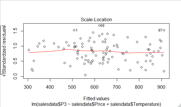
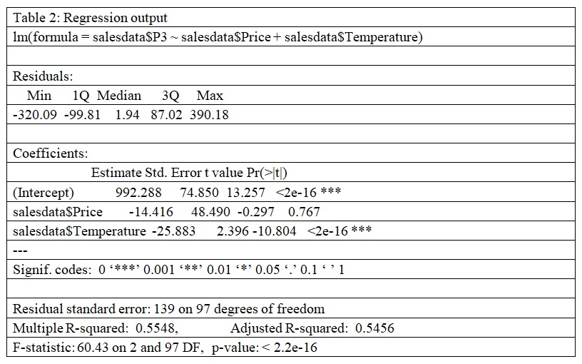
Regression analysis indicates that price and temperature accounts for 55.48% of the variation in the sales of product 3 (Figure 17 and Table 2)
Product 4
Table 3 shows that price and temperature do not account for significant influence on the sales of product 4 (Table 3)
Table 3: Correlation analysis.
Product 5
Time series established that Croston and SBA methods predict variation in sales of product 5 in time series (Figure 18).
Evaluation of Results and Recommendations
Product 1
The calculations of forecasts of product 1 using SES and SMA generated accurate values despite the presence of noise and outliers. As the SMA method achieved lower values for MAE than the SES method, it is a relatively better method. However, the analysis recommends both SMA and SES as a suitable forecasting method.
Product 2
Forecast of sales data for product 2 using the Naïve and Holt’s methods generated accurate values. Holt’s method provided more accurate forecasts than the Naïve method owing to the low MAE values obtained. Additionally, as Holt’s method generates extended periods of averages, which minimize the effects of noise and outliers. In forecasting the sales data of product 2, Holt’s method is fit.
Product 3
The presence of both additive seasonality and trend fits the use of TSEM in forecasting sales data for product 3. The use of the linear regression analysis is appropriate because price and temperature account for 54.48% (R2 = 0.5548) of the variation in the sales level of product 3 (Rosen, 2018).
Product 4
The application of correlation shows that price had a higher level of correlation than temperature. The multiple regression analysis indicated that both temperature and price are not statistically significant predictors of the sales of product 4 because they account for 3.3% of the variance (R2 = 0.033). The analysis recommends the use of price and other explanatory variables in predicting the sales of products 4.
Product 5
The erratic demand for product 5 sales fitted the use of both SBA and Croston forecast methods generated the same outcomes. Although SBA provides accurate findings, the report recommends the use of both methods to allow comparisons of trends, seasons, and levels in sales.
Conclusion
The examination of plots and decomposition of time series of data sales (1-5) indicated different structures. As the structure of sales data determined their forecast methods, SEM, SMA, Naïve methods, TSEM, Holt’s method, regression, and intermittent methods were employed to forecast sales data. SEM and SMA were utilized in the forecast of product 1, the Naïve and Holt’s methods in product 2, TSEM in product 3, regression model in product 4, and SBA/Croston in product 5. In error analysis, MAE and MSE were relevant to products 1-4 because they are not sensitive to outliers. In addition, MAPE was employed with the consideration of the effects of noise and outliers. Scaled type of MSE derived from MSE and the mean of squared overage of the demand.
References
Quirk, T. J., & Rhiney, E. (2017). Excel 2016 for advertising statistics: A guide to solving practical problems. Springer.
Rosen, D. (2018). Bilinear regression analysis: An introduction. Springer.