The abstract
With regard to the theories of Photovoltaics physics learned in the course, this report is an attempt to support and rationalize their implications in actuality. The experiment was done specifically to ascertain how various connected units could be coordinated to give a more reliable and controllable functioning. It is from this understanding that this report is based on an attempt of communicating these findings. The experiment involves investigations of several parameters that are important for any industrial processing unit. Therefore, a slight change in these parameters could bring an effect on the current. How these changes could be coordinated to give a more desired aftermath was integral in this investigation. Of these is the output originating from the controller, its ability to coordinate with the desired power supply was investigated, how the current could be made more effective from the controller point of view was important. It was therefore mandatory when investigating this to apply control measures, and such effects of introducing any step change on parameters like connection, the effects of integral actions on the system’s response were key too. The final part of the experiment involved communicating these findings based on performance characterization where graphical representation was important to clearly illustrate these findings. From these series of experiments, it is clear that whenever there is an overlap in functional mechanism meant to regulate a functional parameter then the process would function at optimum if it is regulated within the recommended range. This would also ensure another dependable functional parameter is highly maximized. For each of these experiments, the literature review, the underlying theory, the adopted methodology, the outcomes and their discussions and finally the derived conclusions have been illustrated as per the scope of work.
The Introduction
Current is defined as the transfer of thermal energy between a body and its environment. Panel, irrespective of its state continues to experience curresnt transfer until equilibrium is attained- a state of zero gradient. This transfer of current is known to occur in three ways-conduction and radiation.
Conduction is flow of current between bodies in direct contact with each other. Although the most significant form of heat transfer in solids or between solids in contact are also known to exchange current through conduction. The third form of heat transfer is through radiation that involves transfer of heat through emission and absorption of electromagnetic waves called thermal radiation. Radiation does not require any medium to be communicated as compared to the other two forms of heat transfer; making it particularly important and interesting in the study of thermal physics. Thermal radiations are known to be emitted in the range of 0.1 to 100 microns-this includes the wavelength of visible light.
The Method
 ) digital display meter reading was monitored for several minutes until it reached a minimum value of 0 W/
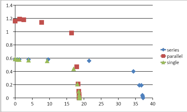
For this lab you will be expected to measure the current-voltage characteristics of two identical photovoltaic panels for the following configurations:
- Series connected panels under full irradiation
- Parallel connected panels under full irradiation
- Single panel under full irradiation, 70% irradiation, 50% irradiation and 10 % irradiation.
In this experimental setup, the method that was utilized involved altering parameters under investigations and measuring their corresponding effects on the arranged changes, these were then compared with the set values so as to generate a flow that could enable regulation of the electrical power supply to heaters. The justifications for this industrial control process are based on the fact that most if not all industrial processes require energy utilization, but of late these have become so expensive that maximum utilization has become a key consideration. There is a need to therefore formulate ways and methods of ensuring such processes attain maximum utilization of the available resources at a controlled approach. Heating applications is the generation and transfer of heat as well as its regulation within set limits to avoid loss of this precious energy. Such settings would more often give a better combination of various parameters under investigations that could be unified to give the best result in any controlled industrial process (Shah and MacGregor, 2005).
For each measurement, you should adopt the following procedure. Move the rheostat to the short circuit position measure the current generated and check to ensure the voltage is zero. Record the results on the appropriate row on the datasheet. This will be the maximum current the panel can generate, therefore select a suitable setting for the ammeter to give a full-scale deflection slightly larger than this value(Mondie, 2005).
Open the open circuit switch and record the voltage and current in the appropriate row on the data sheet. This will be the maximum voltage that the panel will generate. Close the open circuit switch(Zhang, 2010). Increase the load applied to the panel by gradually twisting the knob on the rheostat. You should observe that the voltage starts to rise. Take readings of the current at the voltages indicated on your data sheet.
The Results
The resistance of the resistor and capacitive resistances determine the shape of this graph. At low voltage, the resistance of the resistor is much less. At extreme voltage, either high or low, the impedance is larger and the amplitude of the current is therefore small.
It can be seen that the ideal values and the experimentally determined values are similar. This authenticates the derived results. Graph depicts this variation between the sample and the experimentally determined values of (Sin2 Θ * Qb). The obtained linearity again suggested the successful determination of the calculated values of plot. The plot is largely linear although at larger distances, assumes an exponential form.
The same apparatus and sample test results were used as in parallel Experiment. The graph is plotted that depicts the variation of voltage along the Y-axis. The patch followed by the plot shows a linear trace but with a negative slope. The equation of the trend line was derived to be “y = -0.06x +1.335 with a gradient of -0.06 and a Y-intercept of 1.335 with the positive Y-axis. This magnitude of the Y-intercept suggests the possible values of voltage when current approaches very small values which means that as that the distance from the source of radiation decreases, the intensity of radiation increases; this is also what the inverse Square implicates.
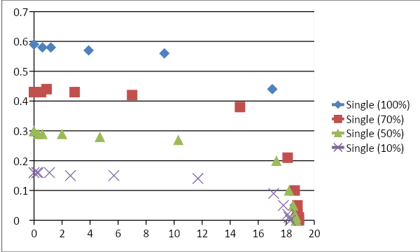
The observations for single largely suggest closely similar values for the view factor although some deviations are encountered. The relationship between voltage and current is plotted in the Graph. The resulting plot assumes a linear approach as the magnitude of voltage begins to rise; this is an indication of the success of the experiment. The derived trend line follows the equation “y = -0.013x + 0.637 with a negative gradient of 0.013 and a Y-intercept of 0.637 with the positive axis.
At lower values of voltage though, deviations are observed where the graph follows a steep form, which could be due to very high values of current flow at smaller amounts to the ambient temperature i.e at the very close separation between the source of radiation and the radiator. The magnitude of the Y-Intercept is similar to the highest of Rc values in the table. This indicates the maximum heat flux at very small differences between the temperatures of the heat source and the radiator. Also, the influence of external factors that could potentially bring about alterations to the desired results in a laboratory cannot be ignored (Dale and Fardo, 2009).
Discussion of results
These experiments were subdivided into six areas of investigations these were; flow rates, power, bandwidth change, stepwise control, and temperature changes. From the first setup involving the flow rate, results show a significant variation in the functional graphical deduction. In the first part, where the flow rate is compared with power and temperature, the flow rate increased when a certain minimum temperature was kept constant, while the maximum temperature declined linearly at constant power. When the flow rate was maintained at a constant value, the minimum temperature rose steadily before it started declining while the maximum temperature declined steadily until it leveled with the minimum temperature. Inflow rate 4 the maximum attained rate for both the channels was at around figure, the channels gave reverse figures, because at no one point did they give a uniform result. These representations however gave a bigger margin in between the settings that were being investigated. The series flow rate of the variables gave a better result only inferior to the first example above. The maximum figure was recorded at figure 0.58, they recorded a lower value of 0, as one increased the first variable the second one declined and that’s why the graph has taken the figure represented by these findings. The third set up herein is referred to as the flow rate 2, whose variations were almost constant; the preceding representations did not have such kind of representation (Lewin, Seider and Seade, 2002). The most notable and observable difference is that the figures gave a less difference in these variations, smaller than the previous two. This showed an improved efficiency in not only timing but also giving the output of the required variable. Similar results to this setting were obtained in the sixth experiment within the flow rate, although the highest variable was achieved at positive nine, another difference is the presence of a wider gap between the functions that represent the utility of the applied variables under control and comparison.
In the fifth setup, (flow rate 8), the functional variables that were examined were also more dependent on each other than in the previous experiments, the gap between the functional variations does indicate more dependent and significant adaptations upon alteration to affect the changing parameters. The last setting stands out because the variables that were investigated did not predict steadiness as expected. These wide differences in the aftermath produced a more unpredictable representation.
From the power experiment, several experimental designs were carried out. In the first setup (power 0.2), a constant variation was seen on channel A, while B gave a slightly noticeable drift; these kept varying by going down until a maximum value was recorded. In Power 0.4, a steady and more variable characteristic was witnessed; this stood out from the first case because there were no variations from the set targets upon which the values had to range. However, more variation was seen in the power 0.6 experiment, where two maximum ranges were gotten at two different value ranges. For the power 0.8 setting, what we see is a different kind of result in that the variations got were not only steady but also uniform throughout.
In the setup named power 1 which assumed a more or less steady distribution and showed a steady variation between the experimental variables, the maximum value ranged within the graphical value. From this, the least recorded variation between the two was noted at around -9.5. This alludes that these variables can be combined and monitored at a certain interval and controlled to ensure the correct values are fully utilized.
From the experiment on temperatures and the bandwidth, an increase in temperatures lead to a decline in the proportional bandwidth, at proportional bandwidth 40, we see a drift in both A and B, they took a uniform drifting. The maximum value for B was much more than that for A, the opposite is true for the lowest value recorded where the minimum for A was lower than that for B. For the positive or negative variable, B was on the positive scale, therefore giving a positive value while A was below the X-axis, this gave a negative value in the entire experiment. In an experiment at proportional bandwidth 60, the maximum for B was 5.5, while for A was 1.8. The experiment gave a similar graphical representation as to the previous one because B variables gave positive values as opposed to A which gave negative values. However, these variations were on a linear scale. Perhaps, the value for A is the lowest for the entire experimental setup. For the experiment at proportional bandwidth 80, the maximum B value recorded was 4.3 against A which was 0. The minimum value for B was -1 while for A it was noted as -3. Equally, these variables were distinct because A gave a negative value as opposed to B, which is a positive variable. In at proportional bandwidth 100 experiment, the highest attainable variable for B was 40, while A is 0; the minimum variables recorded for B was-8 while -3 for A. In this case, B gave a lesser variable than A contrary to other settings. These variables varied uniformly along the scale and could be easily controlled to give the desired function in the processing industry. In an experiment at proportional bandwidth 120, the maximum recorded value for B was 3.8 while -2, was the minimum. A gave a maximum of -2 and a minimum of -6 (Richardson, 2004).
The other segment of experimental set up where the measured value was maintained constant together with the set value and this gave a linear increase in the integral value. In the set up integral 0.75, where B was represented with time to deduce its variation, the maximum variation was 2.5 while the minimum recorded was -1.3, the functional representation gave a more pronounced representation that was centered along the scale. When this representation is compared to the next setting integral 0.5, whose minimum value was -3.5 and it’s maximum as 2.5, we see a more pronounced functionality along the axis than the previous one. The last arrangement in this category integral 1, with the maximum of 2.4 and a minimum of negative three, was also pronounced along the axis as the previous ones.
From the last arrangement of the experiment, there are three main sections under investigation in the derivative band functional parameter these include; derivative band 0.1 upon which we observed a maximum at around 2.4 and was less pronounced along the axis, the minimum variable attained was -4. From the set up derivative band 0.2, the maximum figure was at 2.5 value, this occurred at center of the axis, with a minimum of -2. This representation was more pronounced along the axis. The last segment derivative band 0.3 presented a number of functional peak values with a maximum at 2.5 and a minimum at -2.5. The last segment where the measured value and the set values were kept constant gave a linear rising of derivative action(Dale, RP & Fardo SW 2009).
Conclusions
The experiment successfully determined the calculated values of current that were in close proximity with the values of Rc in the sample test records provided. The graph plotted to compare the experimentally determined and the sample values pursued a linear path which also confirmed the success of the experiment. The equation of the trend line was derived to be “y = -0.13x – 0.6” with a gradient of -0.13 and a Y-intercept of 0.6 with the negative Y-axis.
The Inverse Square Law was successfully established in the experiment as the linearity of the obtained curve in Graph G2 was as expected due to the inverse variation of the area of the transfer intensity with the square of the distance from the center of the source of power. As it can be seen from Graph G2, the plot between the distance from the source of power and the value of sample Rc provided resembles a “y=1/x” hyperbola. This is the reason why the shape of the log curve tends to follow an inverse straight line.
The experiment successfully validated the Stefan-Boltzman Law as the determined values of the view factor F were obtained to be majorly similar. The near-linear plot of the fourth power of the ratio of the emitter temperature to the ambient temperature and the corrected heat flux Rc also suggested the success of the performed experiment.
The experimental values of thermal conductivities of the specimen materials provided were successfully calculated and the graphs depicting the variation of temperature with change in distance from the thermocouple T1 were also successfully plotted.
Findings indicated that maximizing power usage will depend on overlap mechanisms that are laid in place to ensure the regulated temperature is kept within the required range. Such alterations have been found to be instrumental in making the plants effective, safe and environmentally friendly for the people carrying out the exercise in the processing plant.
- A steady deviation in the mains voltage was brought by a decrease in the bandwidth, equally. Changes in measurable temperature were observed once a stepwise change in the set variables was adjusted outside the target limits.
- A rise in the efficiency value of the controller was witnessed due to a decrease in energy produced; this was reflected in an increased flow rate.
- Comparison of these findings to the manufacturer directives as per the manual specifications was important to arrive at the conclusive parameter combinations that gave an ample specification for the various variables.
Reference List
Dale, RP & Fardo SW 2009. Industrial process control systems. Boca Raton: Fairmont Press, Inc.
Lewin, DR, Seider WD, Seade, JD 2002. ‘Integrated process design instruction.’ Computers and Chemical Engineering, vol. 26, no.2, pp. 295-306.
Mondie, S (ed.) 2005. System, structure and control 2004. , Oxford: Elsevier-IFAC.
Richardson, P (ed.) 2004. Improving the thermal processing of foods. Cambridge: Woodhead publishing ltd.
Shah, LS & MacGregor, F. J. (ed.) 2005. Dynamics and control of process systems 2004. Oxford: Elsevier-IFAC.
Zhang, P 2010. Advanced Industrial Control Technology. Oxford: Elsevier.