Machine Learning and Variational Autoencoders

Machine Learning: An Introduction

Machine learning (ML) is one of the most rapidly expanding artificial intelligence branches with far-reaching consequences for technology, computer science, and the contemporary world. The phrase is understood as the concatenation of the meanings of the terms “machine” and “learning.” Therefore, in order to comprehend what machine learning is, it is important to define the terms “machine” and “learning.” On the one hand, a machine is an artificial, non-human entity such as a device or an apparatus that uses such forms of power as electricity to perform a given task or tasks. They typically have several parts or components with definite but interdependent functions that work together to render the entire device or apparatus useful. A computer is an example of a machine, but it can also be used as a component of another machine. On the other hand, “Learning” refers to knowledge acquisition or the process of gaining a skill or an understanding either through training or personal experience. The knowledge gained through learning can facilitate behavioral changes by streamlining them.

Based on the above, ML can have several meanings depending on one’s perspective. For one, it could refer to the process through which computer-based devices and apparatuses utilize existing data to acquire knowledge and improve their predictive accuracy with the passage of time (Burkov, 2019). ML could also denote the deliberate development of applications that, instead of relying on explicit programming, use data to learn and improve operational effectiveness over time. In this regard, machine learning is a computerized data analysis method automating analytical model development by helping computers recognize patterns from existing data and make relevant and accurate decisions without human supervision (Fradkov, 2020). Training in humans occurs through formal processes such as schooling or informally through such one-on-one interactions as apprenticeships. In machines, learning is facilitated by sophisticated algorithms and neural networks that improve a device’s computational powers over time. The algorithms – well-dined and finite implementable computer instructions – use sample or training data to mathematically model phenomena and their accompanying relationships and interactions to help computers make decisions as if they were rational beings.

Although machine learning is now a popular part of computer science, it was not always thought to be possible. Not surprisingly, machine learning has its origins, not in computer science but in psychological research. Significant work that led to the development of ML started with attempts at creating a prototype of the human brain to understand how it functions, particularly how it acquires knowledge and skills from stored information (Fradkov, 2020). In 1949, the Canadian psychologist Donald Olding Hebb, Fellow of the Royal Society, created a human brain model in his book “The Organization of Behavior.” In it, Hebb presents his theories on neuron communication and neuron excitement, noting that “when one cell repeatedly assists in firing another, the axon of the first cell develops synaptic knobs (or enlarges them if they already exist) in contact with the soma of the second cell” (Hebb, 1949, p. 63.). Other developments in the 1950s that paved the way for ML as currently constituted include the creation of a checkers-playing computer program by IBM’s Arthur Samuel in the 1950s and the invention of the perceptron by Frank Rosenblatt in 1957.

Autoencoders

As noted earlier, neural networks play a critical role in machine learning by driving the artificial acquisition of decision-making data by machines. Autoencoders are examples of neural networks used in machine learning. They are unsupervised systems that attempt to encode latent-space inputs and decode them backs. In this regard, they are an approximation of the principal component analysis (PCA) and the t-distributed stochastic neighborhood embedding (t-SNE). However, unlike PCA and t-SNE, autoencoders are extendable into generative models.

Autoencoder Architecture

Although autoencoders perform seemingly complicated tasks, their operational principle and architecture are relatively simple. The unsupervised learning algorithm underpinning the autoencoder applies backpropagation to the training data. It has the encoding function that outputs the latent representation of input and a decoding function that computes the reconstructed information (Bank, Koenigstein and Giryes, 2020). The loss function, which is also present in autoencoders, measures the variability between the original and the reconstructed data. Since the backpropagation aspect of this unsupervised neural network sets target outputs to be the same as the inputs, its mathematical model is in the form . Essentially, the autoencoder tries to master the identity function 

 so that its output is almost similar to the input. Recall that autoencoders have a decoding function that retrieves and constructs the compressed data, i.e., activates hidden unit 

, and is denoted by 

. Unfortunately, this notation fails to capture the explicit expression of the input 

. To resolve this problem, the expression can be re-written as 

, which now denotes the hidden unit 

 for a network with the input 

. Assuming that the hidden unit 

’s average activation 

 is given by:

Then, it would be possible to enforce – approximately – the  constant, where the letter p serves as the sparsity parameter, which is typically close to zero. For example, if it is desired that the hidden neuron 

’s activation is 0.05, an extra penalty term is needed to ensure the hidden unit 

 is always close to zero. The penalty term penalizes any 

 that deviates significantly from 

. Any selected penalty term that gives reasonable results is desirable. An example of the penalty term based on the Kullback-Leibler (KL) divergence is given by:

Where  represents the hidden layer’s neuron amount and the 

 index sums over the network’s hidden units. Notably, the full derivation of the mathematical formulas and models for the autoencoder algorithm, which results in gradient descent, is beyond this paper’s scope.

How the Autoencoder’s Encoder, Hidden Layer, and Decoder Work

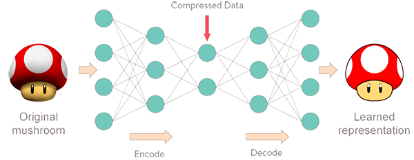
The encoding, hidden layer, and decoding functions of the autoencoder work together to produce the desired outcomes. Encoding works by reducing the dimensions of the input data (Bank, Koenigstein, and Giryes, 2020). In an unsupervised way, the neural networks learn to copy their inputs to their outputs under some predetermined constraints. For example, the autoencoder could limit the latent space’s dimensionality or add noise to the input. The hidden layer works by assigning codes to the input data, thereby significantly compressing it and reducing its space requirements. Finally, the decoder converts the information in the compressed data back into something similar to the original. It works by comparing the encoded data with the decoding script in its memory and substitutes the encoded data with their equivalents. Notably, with its various functions, the autoencoder does its job well by finding efficient data representation approaches. For example, the network could learn and acquire the essential features of a physical entity and drop irrelevant or unnecessary information.

How Autoencoders Compress and Decompress Data

As noted, autoencoders compress data by using the encoding function and decompress them by using the decoding function. The encoder compresses data by converting it into a latent-space representation, which removes some aspects of the data, such as three-dimensionality (Shukla and Fricklas, 2018). Notably, the latent space represents data by putting similar points closer together and less-similar ones further apart. Ideally, by grouping similar data points, the latent space of the autoencoder can identify the features that make these pieces of information comparable and use that information in future decision-making (Sánchez-Morales, Sancho-Gomez and Figueiras-Vidal, 2021). The latent space also finds the simplest and most effective ways of representing data to facilitate analysis. The decompression of data happens when the autoencoder’s decoder reverses the data encoding process. As shown in Figure 1, some information may be lost when decoding compressed data.

Types of Autoencoder Loss Functions and When to Use Them

Most often, the loss function is a mathematical function of the form . This type of the loss function is used when the p-dimensional output of a neural network is compared to some expected outcomes or correct answer. Minimization of the loss function value is achieved by running an optimization algorithm (Sánchez-Morales, Sancho-Gomez, and Figueiras-Vidal, 2021). Other types of the autoencoder loss functions include the squared 

 norm, and the cross entropy. The 

 norm may be represented by 

, while the cross entropy may be notated as 

. The three categories of loss functions include autoencoder losses, linearity losses, and cross-mapping losses. When the intention is to reconstruct the input data as accurately as possible, one could also utilize the Kullback-Leibler (KL) divergence and the Mean squared error loss functions.

Advantages and Disadvantages of Autoencoders

The advantages and disadvantages of autoencoders vary depending on the specific autoencoder type involved. Examples of some types (flavors) of autoencoders in use today are vanilla, sparse, denoising, contractive, and variational autoencoders. A general advantage of all of them is that, as unsupervised intelligence models, they are trainable without labeling (Shukla and Fricklas, 2018). Autoencoders can also reduce data dimensionality and space requirements. It also reduces the time needed to learn data in each available case. Notably, the autoencoder’s backpropagation is compact and allows for speedy coding. Unfortunately, the autoencoder leads to the loss of information. Because the system is trained to ignore some signal noise, the minimization of these losses would depend on the effectiveness of the optimization function.

Where Autoencoders Can Be Used

As unsupervised neural networks, autoencoders have usefulness in a variety of applications. One of them is in the reduction of the dimensionality of any given data. Dimensionality reduction is the process of transforming or reducing data from a high to a low dimensional space without losing the original data’s intrinsic qualities. One reason for dimensionality reduction is circumventing raw data’s curse-dimensionality-induced sparseness, which negatively impacts data analysis. Data which is not dimensionally reduced can also be computationally intractable. Another area of application of autoencoders is denoising (i.e., the identification and elimination of unnecessary pieces of information from a dataset). It is also possible to detect anomalies and generate a new set of data through the use of autoencoders. Anomaly detection occurs when the autoencoder trains the neural network on normal data samples. Similarly, since outliers cause huge reconstruction losses, the autoencoder will flag them as anomalies.

Variational Autoencoders

There are about seven different autoencoder types, and the variational autoencoder is one of them. Unlike the other six types, variational autoencoders assume strong cases for latent variable distribution (Zhao, Song and Ermon, 2017). Its approach for learning’s latent representation causes an additional loss component that may reduce its workings and effectiveness. The approach also introduces the Stochastic Gradient Variational Bayes estimator – an additional training algorithm estimator. As such, the system’s latent vector probability distribution often matches the training data more closely than the standard autoencoders’ do. There is significant control in how one wants to model the latent distribution in variational autoencoders than in others. After training the system, it is also easy and convenient obtaining samples from the distribution and decoding them to generate new data. The main drawback here is that while training the variational autoencoder model, calculating network parameter relationships compared to the output loss is crucial but requires extra attention.

Differences with Standard Autoencoders

The variational autoencoder is different from the standard encoders in many ways. For example, when it is furnished with some input, the variational autoencoder can develop encoding distributions. For example, if the input provided is about a fraudulent money laundering case, the system’s encoder would create a distribution of possible encodings representing the most critical aspects of the transaction. After that, the decoder would turn all the distributions back to the original input about the fraudulent case. In this regard, variational autoencoders allow for data sampling and training the classifier to identify different cases similar to the original input. Notably, the variational autoencoder is effective because it has two (as opposed to one in the standard autoencoders) compressed vector representations. One of these vectors is for the mean encoding, while the other is for this encoding’s standard deviation.

Architecture

The working of the variational autoencoder is similar to the standard one. It is underpinned by an unsupervised learning algorithm that backpropagation to the training data. It also has the encoding function that outputs the latent representation of input and a decoding function that computes the reconstructed information (Khoshaman et al., 2018). It differs from other autoencoders in that it can generate its own data. Therefore, its architecture represents that of a true generative model. Given the input x, the variational autoencoder tries to find the function f so that the equation x=f(x) would be true. The architecture of the variational autoencoder lacks the overfitting tendency. In other words, the system does not try to introduce a sufficiently sophisticated encoder-decoder pair that perfectly maps the training data to a single variable and back, achieving lossless data encoding and decoding. Although a perfectly successful, loss-free data compression and decompression would represent significant mastery of the process, it would not result in any useful information that could be used for predictive applications. As shown in Figure 2, instead of producing the normal latent space’s z point, the variational autoencoder’s encoder creates a distribution N(μ,ϱ), where μ is the “means” parameter and ϱ the standard deviation.

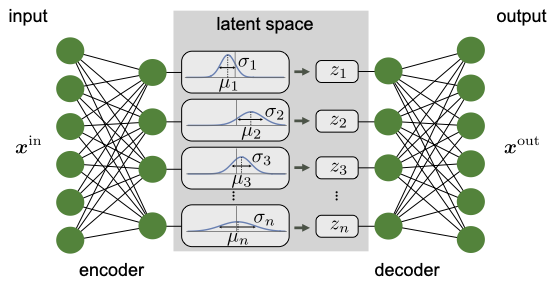
The Mean Vector (Mu, μ)

One of the vectors that the encoder in the variational autoencoder should produce is the mean vector, represented by mu (μ). It is one of the deterministic functions of the inputted data that represents the distribution (Wang et al., 2020). Since the variational autoencoder is the only true generative model of the autoencoders, the mean of the distribution. It provides critical characteristics of the distribution and helps in predicting outcomes. As such, if one can use some measure to classify two input data points as close, their latent space images should also be close. Therefore, the mean helps to solve the question concerning the preferable and effective way of representing the data. The mean is a measure of the output’s central tendency.

Standard Deviation Vector (Sigma, ϱ)

The standard deviation vector measures the extent to which the output data is dispersed from the mean. As such, it indicates the output data’s absolute variability, which is a good indication of the accuracy of the output compared to the input data. The dispersion is high when the standard deviation is great and vice versa. From the distribution whose mean and standard deviations have been calculated, the system could sample the decoder’s input. The distribution used in this regard is given by Z N(μ,ϱ). The formula allows the system to reconstruct various possibilities and possible variations of the original input. After that, the system compares the results with the original inputted training data. Therefore, both the mean and its standard deviation, represented by mu and sigma, respectively, are useful in determining the nature of the distribution of the variational autoencoder’s output.

Sample Layer Vector

The idea behind the development of the variational autoencoder is to have nominal (factorized) distribution points as opposed to one exact copy of the input data in the latent space. For this reason, the variational autoencoder’s encoder has the two vectors mentioned earlier (i.e., the mu and sigma vectors) and a standard loss function. In addition to that, the system has a sample layer vector acting as the regularization term. It is such that the encoder’s distributions are closer to , which is a standard normal distribution. It regularizes the system training by introducing noise in the same way that the dropout layers of the computational neurons do. Notably, the sample layer vector regularization in the variational autoencoder increases generalizations generically and enforces the latent space’s desired structure.

Kullback-Leibler Divergence

The Kullback-Leibler divergence, which is also sometimes called relative entropy or information divergence, is a component of mathematical statistics that is useful in autoencoders. It measures the difference between two probability distributions over the same variable (Kingma and Welling, 2019). It non-symmetrically measures the difference between two probability distributions  and 

 by denoting divergence from 

. This difference, which is generally denoted by: 

, shows an approximation of the information lost when 

 is used in 

 estimation. Specifically, it measures the expected amount of additional bits that programmers require to code 

 samples using 

 code. In the typical cases, 

 is the “true” case of data distribution and observation, and 

 represents a 

 model, theory, approximation, or description. Even though the KL divergence measures the “distance” between two probability distributions, it is neither metric nor symmetric. As such, the KL from 

 to 

 is not the same as the KL from 

 to 

.

Use Cases of Generative Models

Generative models such as the variable autoencoder have numerous natural and hypothetical use cases. For example, they are helpful in applications that predict the next word or phrase in an incomplete sentence. The system predicts with some degree of accuracy the probable next word or phrase in a sentence by giving a sequence of words some probability figures. Over time, these predictive models become more accurate as they learn from their continuing interactions with users. Generative models can also be used in speech recognition and personal assistant software such as Amazon’s Alexa.

Reference List

Bank, D., Koenigstein, N., and Giryes, R. (2020) ‘Autoencoders’, Foundations and Trends in Machine Learning, 3(7), pp. 295-322

Burkov, A. (2019) The hundred-page machine learning book (Vol. 1). Toronto, Canada: Andriy Burkov.

Fradkov, A. L. (2020) ‘Early history of machine learning’, IFAC-Papers On Line, 53(2), pp. 1385-1390.

Hebb, D. O. (1949) The organization of behavior: a neuropsychological theory. New York: John Wiley & Sons

Kingma, D. P., and Welling, M. (2019) ‘An introduction to variational autoencoders’, Foundations and Trends in Machine Learning, 12(4), pp. 307-392

Khoshaman, A et al. (2018) ‘Quantum variational autoencoder’, Quantum Science and Technology, 4(1), pp. 12-39

Sánchez-Morales, A., Sancho-Gomez, J. L., and Figueiras-Vidal, A. R. (2021) ‘Complete autoencoders for classification with missing values’, Neural Computing and Applications, 33(6), pp. 1951-1957.

Shukla, N., and Fricklas, K. (2018) Machine learning with TensorFlow. Greenwich: Manning.

Wang, J. et al. (2020) ‘Thirty years of machine learning: the road to Pareto-optimal wireless networks’, IEEE Communications Surveys & Tutorials, 22(3), pp. 1472-1514.

Zhao, S., Song, J., and Ermon, S. (2017) ‘Infovae: information maximizing variational autoencoders’, Foundations and Trends in Machine Learning, 8(6), pp. 301-360