Introduction
In research work, scholars more often than note collect more than two sets of variables. In situations where two variables are collected and used for analysis, this has been termed as bivariate analysis. Typically the aim of doing this is to establish causes or relationships between the variables (Pallant, 2007). The variables under investigation are the independent and dependent variable.
It is worth noting that the association between the two variables is purely based on how they simultaneously change together-co-variation. To accomplish this, 93223.sav that was attached will be used for the analysis. The major technique to be used in the analysis is cross-tabulation and chi-square using phi and Cramer’s V. It is important to remember from the onset that cross-tabulation is nothing but the merging of the frequency distribution of two or more variables in a single table. This helps the reader to clearly understand how one variable relates to the other. With Chi-square, this is employed to find out whether the observed association is statistically significant (Malhotra, 2010).
Univariate description of the variables
The two variables that are analyzed in this assignment to establish existence or absence of association are limiting long term- illness and age of the respondent. The assumption guiding the link between the two variables presumes that the age of an individual is somehow associated with some kind of illness as one becomes older. It has been shown especially in American society and for that matter across the globe, that much older individuals are suffering from certain illness such as high blood pressure, stroke among others.
The major reason although it might be tied up to poor diet, lack of exercise, genetic or hereditary factors, the age plays a vital role. It is worth noting that the univariates used in this analysis can not be described by any other means other than carrying out a univariate analysis. This has been deemed the simplest quantitative analysis which is done on a single variable and its associated attributes. The main interest is to establish certain basic statistic attributes such as mean, median, mode, standard deviation, frequency and percentages.
Concerning the age of the respondent, the best statistics to explain the variable is average statistics which entails mean and median. To measure the spread of age then the standard deviation was deemed fit. From the analysis, it is evident that there was no missing data in this variable. Additionally, the mean age of the respondent was 38 years (38.56 years). This means that considering all the respondents, the average age was 38 years.
On the other hand, statistics carried out shows that the median age was 38.0 years. Similarly, the standard deviation of the respondents’ age was 12.42. This measure of the spread shows that the age of the respondent varied by12 (12.42) years from the mean. It was also interesting to establish the symmetry of the respondent age. To do this a skewness test was carried out. The skewness stood at 0.235 and the standard error of skewness is 0.016. From the generated graph, the data is skewed to the left. This thus means that majority of the respondents were 45 years and below.
Having in mind that age is associated with limiting long-term illnesses; a univariate analysis of the later variable was carried out. There was no missing data for this variable. From the analysis, it is apparent that 22,236 representing 96.4% of the respondents were not suffering from any limiting long-term illnesses while 830 individuals who represent 3.6% were suffering from limiting long terms of illness. Table 3 summarizes this.
Discussion of any recoding and the rationale for the recoding
It is important to carry out the recoding of data with the main rationale of reducing the volume of data and avoiding sparse tables, the variables limiting long-term illness used in this analysis does not need to be recoded, age as a variable needed to be recoded so that representation and interpretation of the results would be possible. Recoding or binning of data follows the rule of thumb in tables where there should be no more than 20% of cells with a count of less than five (Honaker & King, 2010). The major strategies for doing this include equal interval or equal data. The one to be used in this case will be an equal interval category.
The major steps involved in binning include selecting transform/visual binning/banded, then the variable to be binned is dragged into variables to bin box. Then I clicked continue where the variable in the scanned variable list box is clicked on, click on make cutpoints after this select equal width interval option button followed by setting the value of the first cutpoints location to one less than the minimum variable value displayed in the visual binning dialogue box. Then I entered the cutpoints required clicking on the width box makes the equal-interval to be calculated automatically then I clicked on apply. After doing this I proceeded to make the label by entering a name for the new variable and finally I clicked on the OK button. Switching to the variable view sheet, I cross-checked the decimal and measure information related to the variable.
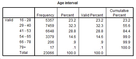
After binning or branding the data on the age of the respondents, the following table gives a summary of the frequency
Table 1 Age of respondents (‘Equal interval’)
Discussion of the observed relationship between the variables
For the relationship between age and limiting long term illness to be established, then an appropriate statistic deemed fit to, was cross-tabulation. It is important to note that the strength of the association, as well as the direction of the association, were of interest. This called for a Chi-square analysis to be performed. Cross tabulation is the merging of the frequency distributions of two or more variables in a single table (Malhotra, 2010).
This helps analysts and other users to understand how one variable relates to another. On the other hand, Chi-square using Phi and Cramer’s V is objectively to assess if an observed association is statistically significant (Babbie, 2009). Both Phi correlation coefficient and Cramer’s V help in understanding the strength/degree of association between variables in question.
From the cross-tabulation analysis, it is apparent that a higher per cent of individuals between 16 and 53 years stated that they were no suffering from limiting long term illnesses. On the other hand, individuals above 54 years old had a higher percentage of suffering from limiting long term illnesses (Table 2). Biologically, older members of the society are prone to serious illnesses and even if they are under medication, their chances of getting completely healed are very minimal (Wootton, 1997).
Why use Chi-square
The rationale of using chi-square test, it establishes a relationship between two variables. However, unlike correlation, it goes an extra mile in explaining not only the direction of the association, strength of the association but also it compares observed and expected data (Pallant, 2007). From the Chi-Square table, it is apparent that the association between age and limiting long-term illness is statistically significant (Cramer’s V = 0.122, X2(5) = 342.010, p=0.000). (Table 5) Thus the hypothesis held initially as one grows older, there are higher chances of suffering from limiting long term illness. This can be due to lower immune systems.
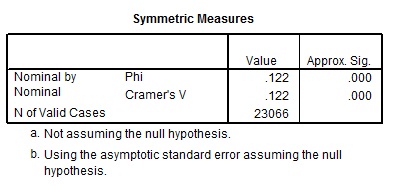
When considering the degree or strength of the association, Cramer’s V value explains this so well. From table 3, V=0.122. Based on the guidelines put forth the association between the two variables (age and limiting long term illness) weak and positive (Malhotra, 2010).
A graphical representation of the association
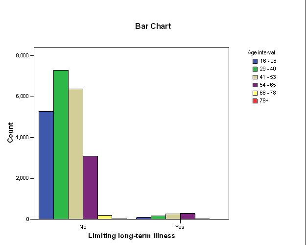
From the bar graph in Fig. 1 and based on the respondent response, it is apparent that the majority of older individuals or ageing are suffering from limiting long term illness. On the other hand, the majority of individuals less than 65 years old are not suffering from such illnesses.
Impact of measurement error and missing data
Although the variables used had no problem with missing data, it would be rational to clearly explain the implications of measurement errors and missing data. It has been shown that missing data when not properly handled by the various methods such as listwise deletion, zero imputation, and two-way imputation among others will results to variation in bias, errors in root mean squares. In the end, it increases the rates of committing Type I and Type II errors. Measurement errors also have the same effects of generating bias that eventually impacts on the findings and generalization of the results (Honaker & King, 2010).
Conclusion
From the analysis of the two variables, age and limiting long term illness; it is evident that there is a positive weak association between them. Results from chi-square indicate also that the relationship was statistical significance, what this means is that the age dictates where or not an individual will suffer from a limiting long term illness (Cramer’s V = 0.122, X2(5) = 342.010, p=0.000). From cross-tabulation, it is evident that individuals older than 54 years are prone to limiting long term illness as compared to those aged 53 and below.
Appendix
Table 2. Cross tabulation.
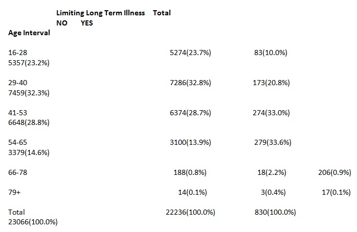
Table 3. Measure of spread and average (age).
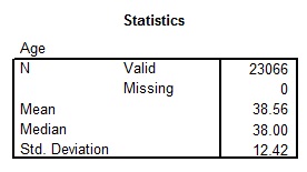
Table 4. Chi-square test (Agebinned and Limiting long term illness).
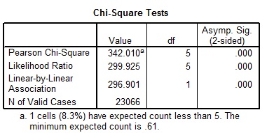
Table 5. Symmetric Measures.
References
Babbie, E., 2009. The Practice of Social Research. New York: Wadsworth Publishing.
Honaker, J., & King, G., (2010). What to do About Missing Values in Time Series Cross-Section Data. American Journal of Political Science 54(2): pp. 561–581.
Malhotra, N., 2010. Marketing Research, An Applied Orientation. Pearson Education, Upper Saddle River, New Jersey.
Pallant, J., 2007. SPSS Survival Manual: A Step-by-step Guide to Data Analysis Using SPSS. Crows Nest, NSW: Allen & Unwin.
Wootton, B., 1997. Occupational Employment: Gender differences in occupational employment. Monthly Labor Review, 2(4): pp.15-24.