Free market and mixed economy
An economic system is important in allocating scarce resources. There are several economic systems that have distinct characteristics. In a free-market economy, there are minimal or absence of interventions. The market is controlled by forces of demand and supply. Further, the economy is self-adjusting. Thus, if there is disequilibrium, the market will adjust to correct the disequilibrium. This implies that an external force cannot have control in the operations of the market. On the other hand, a mixed market economy is made up of both the private and public sector. Thus, there is a heavy government presence in a mixed market economy. Basically, the role of government is to provide important commodities that if left in the hands of the private sector, they will not be handled well (Douma & Hein 2013).
A change in quantity supplied and change in supply
The differences between these two aspects of supply are caused by factors that create these movements. “A supply curve can either shift from one position to another, or there can be movements along a supply curve” (Bade & Parkin 2013). A change in quantity supplied arises if there are movements along a supply curve. This movement can be explained by the law of supply. The law states that a rise in the price of a commodity causes an increase in the quantity supplied while holding other factors that affect supply constants. There are several other factors that affect the supply of a commodity (Bade & Parkin, 2013). A change in quantity supplied arises from the direct association between price and quantity supplied. It ignores other factors. The relationship is shown in the graph presented below.
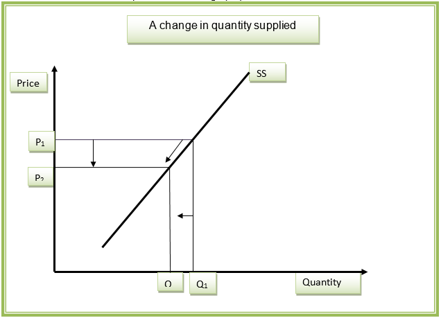
A drop in the price of the commodity from P1 to P2 will cause a movement along the supply curve as displayed by the arrow. This will have an effect of lowering the quantity demanded from Q1 to Q2. Thus, it can be noted that a change in price has an effect on the quantity supplied but not on the supply curve. The supply curve maintains the same position before and after the changes. As mentioned above, other than price, there are several other factors that affect the supply of the commodity. Some of these factors are either endogenous or exogenous variables. For instance, a company can decide to use more sophisticated and efficient machinery in production. This has the potential of increasing output, and it is an example of an endogenous variable. Further, the government introduces a subsidy that lowers the cost of production. This has the potential of increasing the quantity produced, and it is an example of an exogenous variable. These non-price factors make the supply curve to change position, and they cause a change in supply. The graph presented below shows an illustration of a change in supply.
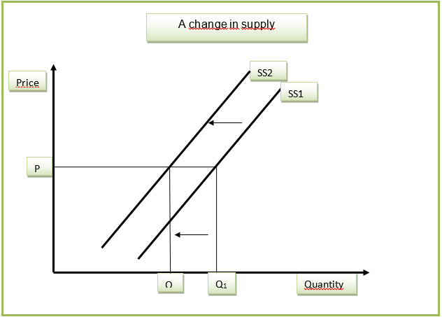
Unfavourable non-price factors will cause the supply curve to shift inwards from the original position SS1 to the new position SS2. This has a negative effect on the quantity supplied. As can be seen in the graph, the quantity reduces from Q1 to Q2. In the graph, it can be noted that the supply curve changes position at the same level of price. There is no price movement during a change in supply.
Cross price elasticity of demand
There are different types of elasticity. Cross price elasticity focuses on the relationship between the two commodities. This type of elasticity gives information on the extent by which a change in the price of one commodity affects the change in demand for another commodity. From a mathematical point of view, this elasticity is calculated through the division of percentage change in one commodity by the percentage change in another commodity. Thus, cross-price elasticity shows how the quantity demanded of one commodity will react to the changes in the price of other related commodities.
Two commodities can either substitute or complement each other. Examples of two complementary goods are rice and beef (Tucker 2010). These two products can be consumed at the same time. If the coefficient of price elasticity is zero, it implies that the two commodities being analysed are not related. Further, if the price elasticity is greater than zero (positive), it implies that the two commodities are substitutes. This relationship is based on the fact that in the increase in the price of one commodity causes the demand to fall. Consumers will move to consume the substitute commodity that retails at a lower price. This cause the quantity demanded of the second commodity to grow. An example of two substitute goods is cantaloupe and watermelon. Further, if the cross-price elasticity is less than zero (negative), it shows that the two commodities are complementary.
These commodities are consumed together. For such commodities, if the price of one commodity increases, the quantity demanded falls. Consumers will purchase less of the complement commodity. This causes the demand to fall. Cross price elasticity is important when forecasting the demand for various commodities. For instance, if the price or quantity demanded of commodity changes, an analyst can be able to monitor the trend of a related commodity (Perloff 2012). This can help management in making decisions that relate to production.
Income effect and substitution effect
The result of a change in price can be disintegrated into these two effects. The diagram presented below shows the income and substitution effect.
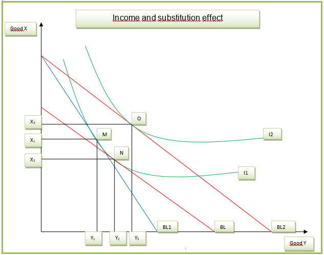
Commodity Y and X will be used to explain these two effects. Based on the law of demand, a drop in the price of commodity Y will cause an increase in quantity demanded. This increase can be broken down into income and substitution effect. In the graph above, “the equilibrium is attained at the point where the indifference curve meets the budget line” (Tucker 2010). The three equilibrium points are M, N, and O. A fall in the price of commodity Y makes the consumer purchase more of commodity Y and less of X. This explains the movement from point M to N. The consumer is substituting commodity X for Y. Point M and N are on the same indifference curve.
This shows that the level of satisfaction derived does not change after the substitution. Thus, the substitution effect of a price fall is shown by the movement from M to N. A fall in the price of commodity Y will cause the real income of the consumer to increase because they can be able to purchase more units of Y. The increase in real income will make the budget line to hinge from BL1 to BL2. This shows a higher consumption level of commodity Y. The consumer will move to a higher indifference curve, I2. The new equilibrium point will be O. The movement from N to O is as a result of income effect (Tucker 2010).
Perfect competition and monopoly
Perfect competition and monopoly have discrete characteristics. First, “in the case of perfect competition, there are no barriers to entry and exit” (Douma & Hein 2013). Firms are free to participate in the market. Therefore, there are several sellers in the market, and they are price takers. However, under a monopoly, there are barriers to entry. This implies that there is only one firm operating in the market and has control over prices. Secondly, the commodities being traded in a perfectly competitive market are numerous and similar. In the case of a monopoly, there is only one commodity that is being traded in the market (Tucker 2010).
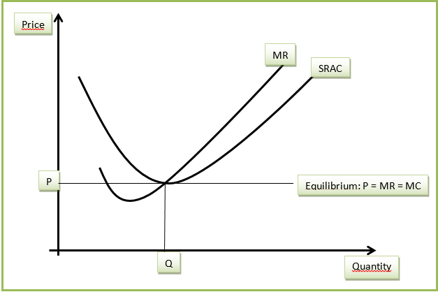
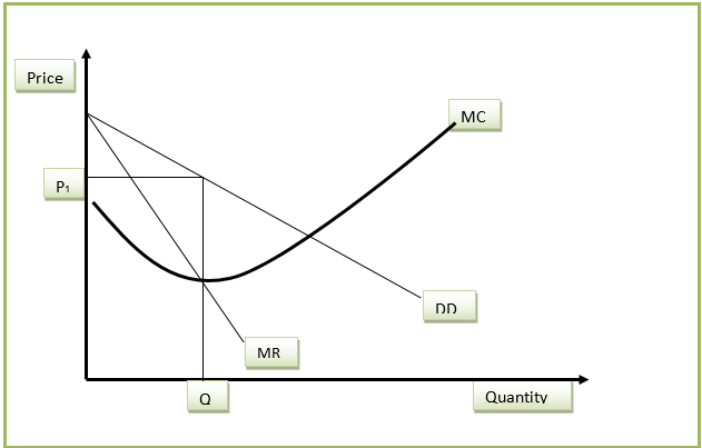
The commodity does not have a close substitute. Finally, the two market structures differ in terms of availability of information. In the case of perfect competition, information that pertains to the production of commodities is available by the buyers and sellers in the market. However, in the case of a monopoly, this information is not readily available. The equilibrium points of these two types of market structures are presented below.
Perfect competition
Monopoly
References
Bade, R & Parkin, M 2013, Essential foundations of economics, Pearson Education Inc., USA. Web.
Douma, S & Hein, S 2013, Economic approaches to organizations, Pearson Education Inc., London. Web.
Perloff, J 2012, Microeconomics, Pearson Education Inc., England. Web.
Tucker, I 2010, Survey of economics, Cengage Learning, USA. Web.