Electromagnetism Studies in Laboratory Works

Words: 2877 Pages: 11

Introduction

One of the four fundamental types of interaction widely found in nature and used by humans in the industry is electromagnetism. In general, electromagnetism should be understood as a branch of general physics that studies the interaction of charges and the electric fields they create with magnetic fields (Braza, 2020). In the theory of electromagnetism, there are a huge number of principles and regularities that determine the behavior of electric and magnetic fields, their mutual formation, and their change under the influence of other factors. In this lab report, the main objective of the study was to explore different aspects of electromagnetism by means of five laboratory works, including several exercises.

Laboratory Work No. 1: Electromagnetism

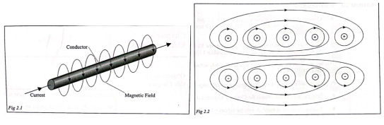
Laboratory Work #1 offered the basics of electromagnetism for study. In particular, the right-hand rule or corkscrew rule (Figure 1) was demonstrated as a valuable tool for determining the direction of magnetic field lines created by the motion of a current. The work also proposed to investigate the Hall effect, an electromagnetic phenomenon that occurs when some sample with a current is placed perpendicular to the magnetic field (Universaldenker, 2022). When this conductor is placed in the sample, a potential difference arises; depending on the material of the conductor, the value of this voltage will differ.

Figure 1: Demonstration of the right-hand rule for a wire (left) and a set of conductors wound into a coil (right) (Laboratory Manual)

Electromagnet

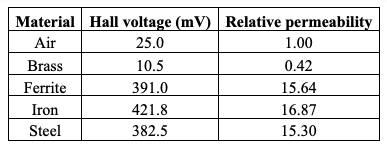
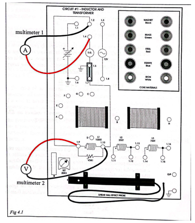
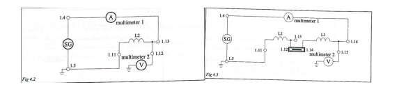
Hypothesis: the basic hypothesis is that each of the core materials affects the magnetic field strength differently, and this difference can be traced quantitatively. Method: an illustration of the board used is shown in Figure 2. As can be seen from the diagram, the coil was connected in sequence with the DC source; the voltage was set to 5 V. The probe was used to determine the direction of the magnetic field lines because, as it was said in the manual, the white point of the probe was maximum when facing the north magnetic pole. Before measuring the magnetic field strength for the different cores, the Hall effect sensor was initially set up with an evaluation of its performance and a flux density measurement for the air gap. The relative Your Last Name 5 permeability of each material was calculated by dividing the corresponding Hall intensity for the material by the field strength created by the air gap.

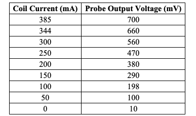
Figure 2: Schematic of the electrical circuit used in the exercise (Laboratory Manual)

Results: Using the right-hand rule, it was determined that as the coil current moved in the direction of 1.9 to 1.10, magnetic field lines were created coming out of the right side (north) of the coil and into the left side (south). For five different coil cores, the corresponding Hall effect values were measured, and the relative permittivity values were quantified. The results of the measurements are shown in Table 1.

Table 1: Results of Hall voltage measurements and relative permeability calculations for materials

Discussion: an investigation of the effect of the nature of the material on the Hall voltage is presented of interest. Specifically, four varied materials and air were used as coil cores. The results of this experiment showed that for each of the materials, the voltage of the generated magnetic field was different, as predicted by the hypothesis. Quantification of the results shows that iron is the best option to place inside the coil because this material is able to maximize the magnetic flux density compared to the alternative materials from the exercise.

Magnetomotive Force

Hypothesis: the hypothesis was that an increase in current led to an increase in voltage on the coil. Methods: the same plateau as in Figure 2 was used as the electrical circuit, but it was adapted in this exercise. The number of turns in the coil was 1000, and the ferrite from the previous exercise was used as the coil core. A current of varying strength was applied to the coil, and the output voltage was recorded with a multimeter probe. Results: the relationship between the current applied to the coil and the voltage recorded was tabulated; Table 2 demonstrates these entries. Fig. 3 shows an almost linear relationship between the measured quantities. It is seen that as the coil current increases, the value of the output voltage measured with the probe increases.

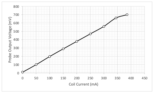
Table 2: Results of output voltage measurements for different coil currents

Figure 3: The linear relationship between the coil output voltage and current, shows a direct proportionality between the two

Discussion: The exercise confirmed the hypothesis that there is a direct proportionality between the output voltage and coil current. Some disturbance of linearity of this relationship with increasing current could be evidence of a thermal effect of the resistance, as follows. The MMF for a voltage of 250 mV can be determined for the plotted graph — to do this, the corresponding current value (125 mA) must be multiplied by the number of turns (1000). Consequently, the MMF for this coil at 250 mV is 125,000 mAT.

MMF To Change Coil Revolutions

Hypothesis: increasing the number of turns in the coil should also increase the MMF. Method: the plateau was adapted for the job, and the L3 coil with ferrite tip was used at 250 mV. The MMF value was measured for a different number of turns in the coil. Results: the corresponding MMF values depending on the applied current and number of turns are shown in Table 3. The average MMF value at 250 mV was calculated to be 148.583.3 mAT.

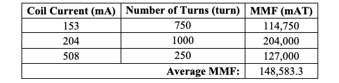
Table 3: MMF calculations as a function of the number of turns and the current used

Discussion: the results showed that there is a natural increase in voltage with an increase in the number of turns, but one cannot ignore the significance of the current strength for this relationship. It was shown that it is possible to determine the average MMF for a given field with such measurements.

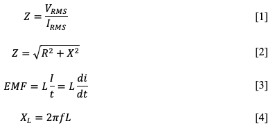
Laboratory Work No. 2: Inductive Reactance When an alternating current passes through an electrical circuit, impedance occurs. The formula for calculating this is shown in Equation [1]. Impedance is a complex characteristic because it consists of two types of resistance, namely the resistance itself and its reactive form, characteristic of coils and capacitors [2]. The resistance of the coil is usually significantly less than the reactive resistance, so in many cases, it can be neglected. In addition, when inducing an EMF in the circuit, the magnetic flux is directly proportional to the current [3] — the reactance, in this case, is calculated by the formula [4].

Reactance Hypothesis: through a series of measurements and consecutive calculations, it can be shown that the inductance of the coil can be determined through the reactance. Method: ferrite was used as the coil core, and the coil voltage was set to 2 V. Current was measured for the circuit and then converted to reactance using the formulas; the ultimate goal was to determine the inductance.

Figure 4: Schematic diagram of the electrical circuit used in control (Laboratory Manual)

Results: the direct measured result was only the exact coil voltage and the measured output current, through which the impedance (310.15Ω) and the inductance of this ferrite-core coil (49.36 mH) could be determined — the results are summarized in Table 4.

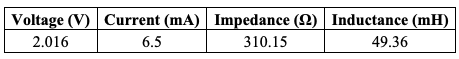
Table 4: Results of measurements and calculations for the exercise

Discussion: The exercise showed that with the measured current, it is possible to determine the inductance value of the coil at a given frequency. It is noteworthy that the determined inductance turns out to be about ten times the resistance of the coil, as follows.

Effect of Core Material on Inductance

Hypothesis: the relative permeability for different materials as coil cores affects the calculated inductance Method: the circuit diagram and the coil voltages are the same as in Exercise 4.1; the difference is in the use of different core options. Results: Since the calculation part of the work was similar to the previous exercise, the results were similar; meanwhile, impedance and inductance results were obtained for each of the materials, as shown in Table 5.

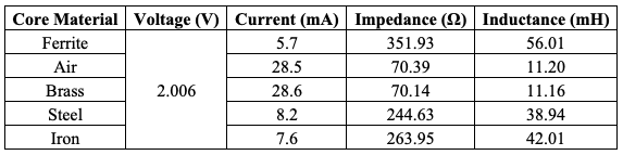
Table 5: Calculations of impedance and inductance depending on the material used as the coil core

Discussion: This exercise showed that the impedance and inductances were highly dependent on the type of material used. The lowest impedance and corresponding inductances were found for Brass, while the maximum performance was shown for ferrite. The difference in the final values is due to the different possibilities of current formation in the circuit — the lowest current was characteristic of the materials that found the highest resistance in the circuit.

Effect of the Number of Turns on Inductance

Hypothesis: the hypothesis was that increasing the number of turns increases the impedance and inductance in the circuit. Method: the procedures were similar to past exercises, but several coils were used in series, as shown in Figure 5. The frequency in the network was chosen to be 1 kHz, and ferrite was used as the coil core. The input voltage was set to 1 V.

Figure 5: Schematic representation of the circuit used for 250 turns (left) and 1000 turns (right) (Laboratory Manual)

Results: by measuring the current at different numbers of coil turns, the reactive resistance and inductance in this circuit can be calculated. The results are shown in Table 6.

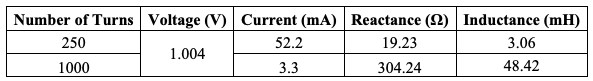
Table 6: Results of voltage and current measurements in a circuit with different numbers of coil turns give different outcomes for reactance and inductance

Discussion: The exercise showed that an increase in the number of turns in a coil results in an increase in the reactance and inductance in that circuit — hence, the hypothesis is confirmed. This data is consistent with what is known, indicating a direct correlation between the number of coils turns and inductance (RSD Academy, 2020). It can clearly be seen that quadrupling the turns increases the inductance by a factor of 16 with minor error (48.96 vs. 48.42), as the Laboratory Your Last Name 14 Manual suggests. Finally, if increasing the turns to 750 (by a factor of three), the inductance is expected to increase to 27.54, nine times the initial value.

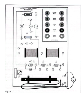
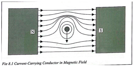
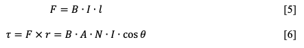
Laboratory Work No. 3: Force on a Conductor and the Motor Principle The presence of a conductor with a current in the magnetic field directly affects the behavior of the magnetic field lines, causing perturbations, as shown in Figure 6. The movement of this conductor is dictated by the left-hand rule, which shows that this conductor must move downward away from the magnetic field (FuseSchool, 2020). The formula determines the force with which the conductor is pushed out of the field [5]. Torque is the force acting in the direction of rotation of the conductor in the magnetic field (Figure 7). The torque can be determined numerically according to the formula [6].

Figure 6: Change in the behavior of the magnetic field due to the presence of a conductor with a current (Laboratory Manual)

Figure 7: Vector representation of torque and force (Laboratory Manual)

Simple DC Motor

Hypothesis: Increasing the voltage in the circuit will increase the rotation speed of the flywheel.

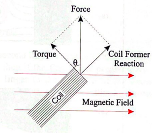
Method: This exercise uses an oscilloscope set to 2 ms/div. The power supply gives a voltage of 5 V to the circuit — when the voltage is applied, the motor starts to rotate according to the left-hand principle. For each revolution of the flywheel, the time was measured, which is numerically equal to the time between two pulses on the oscilloscope.

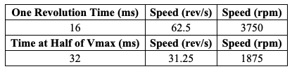
Results: the maximum speed of the motor is reached at 800 mV. For this speed, the time required per revolution was measured, from which the speed in rev/s and rpm were calculated. Similar steps were performed for half of the maximum speed voltage, as shown in Table 7. As can be seen, there is a difference of 0.5.

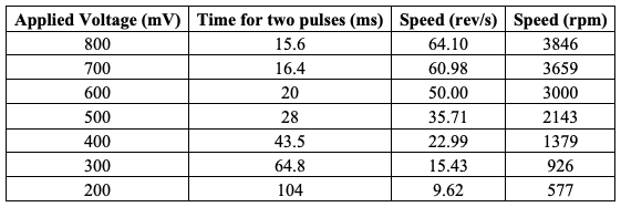
Table 7: Results of time-per-turn measurements at maximum and half voltages

Similar steps were performed to measure time per revolution for seven different circuit voltages; the results are shown in Table 8. Figure 9 shows the dependence of flywheel speed on circuit voltage.

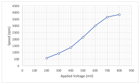
Table 8: Results of measurement of time per revolution at different voltages

Figure 9: Dependence of rotation speed of the flywheel on the voltage in the circuit

Discussion: the completed exercise demonstrated that an increase in the voltage in the circuit leads to a decrease in the time per revolution and therefore increases the speed of rotation of the flywheel — the hypothesis was confirmed. The motor used is allowed to be called linear because the form of its dependence slightly resembles a linear one, and the speed difference between the maximum and half voltage is equal to 0.5.

Back EMF

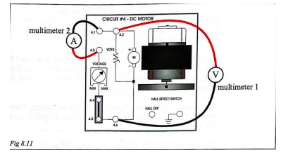
Hypothesis: the rotation of the coil in the circuit causes a reverse EMF resulting in a drop in the total voltage. Method: the tuned circuit was similar to the one used in the last exercise but with a difference in wiring, as shown in Figure 10. The voltage on the motor was set to 200 mV. After the armature resistance was recorded, the motor was started, and the new circuit characteristics were recorded.

Results: the measured armature current was 0.19 A. From this value, at a known voltage (0.22185 V), the resistance of the armature was calculated, namely 1.17 Ω. When the motor started, the applied voltage was 1.590 mV, and the armature current was measured as 157 mA. Then the voltage drop across the armature was calculated as 1.17 Ω ×157 mA = 0.184 V.

Consequently, the inverse EMF was 182 mV.

Discussion: as the coil rotates in the magnetic field, inverse EMF occurs, and this inverse EMF causes a voltage drop in the circuit — the hypothesis is proven.

Laboratory Work No. 4: MATLAB Simulink

Hypothesis: Using MATLAB is appropriate for modeling a single-phase circuit and its automatic calculation.

Method: The laboratory work was performed in MATLAB software with the help of the Simscape Electrical library. Figure 11 shows the circuit diagram that was modeled in the program. The parameters of each block were set according to the instructions in the Laboratory Manual. The circuit was simulated with an end time of 0.1 and a maximum step size of 0.0005.

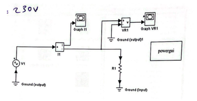
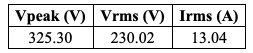
Figure 11: Electrical circuit built-in MATLAB (Laboratory Manual)

Results: The MATLAB simulation under specified conditions determined the RMS voltage to be 230.02 V and the corresponding current to be 13.04 A, as shown in Table 9.

Table 9: Simulation results for a single-phase circuit

Discussion: It is noteworthy that the obtained RMS voltage is identical to what was theoretically assumed, namely 230 V. This confirms the hypothesis that MATLAB can be successfully used to simulate single-phase electrical circuits.

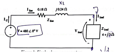
Laboratory Work No. 5: Investigate the Torque/Speed Characteristics of DC Machines Part I Hypothesis: The first part of this exercise will verify that using MATLAB helps to calculate current, peak voltage, and total resistance in a circuit by knowing the VRMS value. Method: this exercise again requires the use of MATLAB software with the Simscape Electrical library pre-installed. An electrical circuit was designed in MATLAB according to Figure 12 – the parameters of each block were set according to the Laboratory Manual. The circuit contained both normal and reactive resistances.

Figure 12: Schematic representation of the circuit required for the design in MATLAB (Laboratory Manual)

Results: Since the initial VRMS value was given in the instructions, the rest of the calculations were done according to the design. Equations [7]-[11] show the sequence of calculations performed.

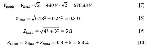
Discussion: calculations have shown that simulation of a circuit with a load allows us to determine the value of total resistance, current and peak voltage in the circuit, knowing VRMS at a given frequency; this confirms the hypothesis. Comparison of the obtained results with those simulated in MATLAB allows us to determine the high accuracy of such calculations. In other words, MATLAB can be used to calculate the characteristics of a simple electric circuit with a load.

Linear Transformer in MATLAB

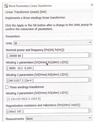
Hypothesis: Open-circuit and short-circuit tests simulated for the linear transformer in MATLAB are the same as theoretically expected. Method: An electrical circuit was built in MATLAB according to Laboratory Manual Linear Transformer settings. An image of such a circuit is shown in Figure 13. The circuit was set to units according to the characteristic in Figure 14. An open circuit test showed with a voltage to the transformer of 8 kV showed the viability of this circuit. In addition, a short-circuit test was also conducted.

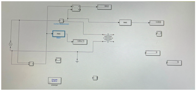
Figure 13: Simulated line transformer circuit

Figure 14: Units used for the line transformer circuit.

Results: The following calculations were used for the simulation:

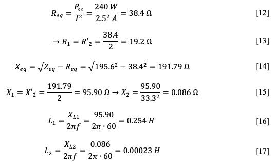
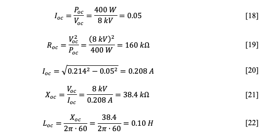
Discussion: The calculations shown above correspond well to what was modeled in MATLAB. Consequently, the hypothesis is confirmed.

Conclusion

The five completed laboratory works showed the diversity of the phenomenon of electromagnetism and demonstrated a thorough understanding of the problem-solving mechanism. Using real circuit design and virtual simulation, circuit calculations were performed. A good correspondence between the calculated and measured quantities was shown, which demonstrates the high quality of the work performed.

Reference List

Braza, J. (2020) The basics of electromagnetism. Web.

FuseSchool (2020) Fleming’s left hand rule | magnetism | physics | FuseSchool.

RSD Academy (2020) Inductors Part 2 — factor that affect inductance. Web.

Universaldenker (2022) Hall effect. An explanation that everyone understands.