Introduction
D. M. Pan seeks to determine whether using square footage is a good benchmark for listing home prices. This report is based on statistical analysis to determine if the square footage of a house is a good indicator of the listing price using real estate data for all U.S. home sales. Linear regression is used when the relationship between the variables is approximately linear.
When using linear regression, the scatterplot will show a somewhat linear relationship between the predictor variable and the response variable. In linear regression, the predictor (x) variable is the variable that is being used to predict the value of the response (y) variable, which is the variable that is being predicted.
Data Collection
A random sample using the RAND function, =RAND (), in Excel. The function was applied to generate a random number between 0 and 1 for each cell in the housing data. After assigning random numbers to each listing, the data was sorted from the smallest to the largest by expanding the selection (Thrane, 2022). The first 50 homes were copied and pasted into a new worksheet to form the sample dataset. The predictor variable is the square feet, and the response variable is the listing price.
The scatter plot shows a possible linear relationship between the listing price and square feet; therefore, the variables are appropriate for developing a linear model.
Data Analysis
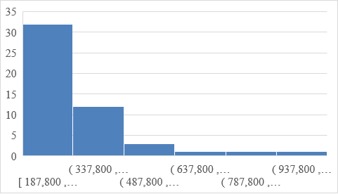
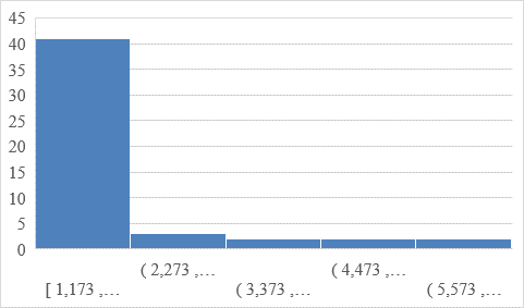
Table 1: Summary Statistics for Both Variables
The frequencies for the listing price and square feet show that most homes have a cost of between $187,800 and $337,800, and they cover an area of between 1173 square feet and 2273 square feet, respectively. Therefore, the shape of the histograms is similar, with a higher frequency to the left, shown by a bigger size that declines in frequency and size to the right. The measures of center and spread (mean, median, and standard deviation) square feet of the homes in the sample are 2194.34, 1849, and 1135.992, respectively. The measures of center and spread (mean, median, and standard deviation) listing price of the homes in the sample is 349922, 316000, and 157202.6, respectively. Higher listing prices and houses with more square feet represent outliers.
The shape of the histograms for the listing price and square feet from the sample of house sales and the national population show an identical pattern. The measures of center and spread (mean, median, and standard deviation) of the listing price and square feet of the homes in the sample and national population are similar. The mean and median square feet difference is 83 and 32, respectively. The difference in the mean and median of the listing price is $7557 and $2000, respectively. The means in the sample are higher, while the medians in the national population are higher. The standard deviations for the sample’s square feet and listing price are also increased by 214 and $31292, respectively. The sample size of 50 is not adequate for a population of 1000, but there is no unusual pattern between the sample and the national population.
Develop Regression Model
The scatter plot shows a linear relationship between the listing price and square feet such that the listing price goes up when the square feet increase. Therefore, the regression model is appropriate for the analysis. The trend line of the scatterplot is upward sloping from left to right and is relatively steep, showing a strong positive linear relationship. The scatterplot indicates outliers represented by higher square feet connecting to more listing prices. The outliers cause the relationship between the listing price and square feet to become stronger (Thrane, 2022). If the outliers are removed, the relationship would be affected such that there would be no direct connection between the variables. The correlation coefficient is 0.91, calculated in excel using the data analysis tool pack. The calculated r value supports the observation from the scatterplot.
Determine the Line of Best Fit
The regression equation is given by y = 72577 + 126.39x. Y is the response variable denoted by the listing price, and x is the predictor variable representing the square feet. The intercept, 72577, means the constant listing price, 126.39 is the intercept. The linear regression has a positive slope indicating the amount by which the listing price increases with a unit increase in square feet. The R-squared for the equation is 0.8342, meaning that the regression model shows a more robust positive linear relationship. Using the regression equation, a home of 1500 square feet would cost; 126.39(1500) + 72577 = $262,162.
Conclusion
In summary, homes with ample space, as measured by higher square feet, are expected the cost more. Therefore, D. M. Pan should determine the listing price using area by square feet, and the price should go up as the square feet increase. The analysis results were expected since using more space to construct a house consumes more resources meaning the listing price should be higher. A location change could support different results, given that regions have varying land and construction costs. An exciting follow-up research question would be; what is the effect of home location on the listing price?
Reference
Thrane, C. (2022). Doing Statistical Analysis. Taylor & Francis.