Philosophical Research: Setting the Scene

Introduction

Psychological research involves the empirical pursuit of exploring and explaining phenomena. We might ask questions such as: Does X vary with Y? Does X cause Y? What is the strength of the relationship between X and Y? Within the context of clinical psychological research, we might ask questions such as: Can we better test for anxiety and maladaptive thinking patterns? Which treatment is better: pharmacological or psychological?

To answer such questions, we need to acquire some knowledge of a given phenomenon, as well as the scientific method that enables us to systematically evaluate observations of the phenomenon. This topic discusses these concepts as well as outlines in broad terms the research approach by which phenomena might be explained.

Acquiring knowledge

There are a number of ways to acquire knowledge. The traditional ‘folk’ methods include intuition, authority and rationalism.

INTUITION: This might be defined as coming to know things without substantive reasoning. Therefore, the knowledge acquired is not always accurate.

AUTHORITY: We are more likely to accept information from an authority structure or a person in authority. However, this information may not be accurate and may amount to little more than propaganda espoused by a structure, system or person with vested interests in presenting the information in that way (e.g. political self-interests).

RATIONALISM: This approach assumes that reasoning and logic will lead to correct interpretations. However, such ‘common-sense’ approaches may also lead to erroneous conclusions. With rationalism, a conclusion is often logically derived from an incorrect premise, such as underpinning stereotypes leading to incorrect interpretations of people and situations such as ‘all poor people are lazy’. Rationalism has its place (even in science in the form of empirical reasoning); however, it is a biased approach to knowledge acquisition when used in isolation.

EMPIRICISM: Empiricism involves direct observation. Systematic observation underpins the scientific method of knowledge acquisition. In order to begin to understand ‘things’ objectively, we turn to the empirical approach.

Science and the scientific method

Science is the objective, systematic process of describing, analysing and explaining phenomena in the form of existence and events, and the relationships between them. Science is not a single entity. Instead, it is a set of best-practice techniques used to accumulate knowledge about what is real. This is based on the premise that there is some order and structure within the universe and that ‘things’ can potentially influence one another. If there is complete randomness, then there is no way to predict occurrences. We know there is not complete randomness, so we can draw upon various scientific methods in research.

There are three main goals associated with the scientific pursuit in research:

• To describe phenomena
• To explain phenomena
• To predict the existence of a relationship or forecast an outcome.

You are likely to come across varying typologies of the scientific method, but the main aspects we consider in this subject are described below.

Scientific method: The main aspects

Observation, systematic and objective methodology

The scientific method involves observing, systematically collecting and evaluating evidence so as to be able to test ideas and answer questions like those above. Systematic empiricism is key here. This involves carefully structured observations and objective measurement (i.e. without bias). As psychology researchers, we may merely observe and measure without interfering in the order of things (an observational research approach such as a survey), or conversely, constrain or manufacture particular conditions or circumstances in order to see the effects (these are quasi-experimental or full experimental approaches where we seek to ‘manipulate’ the way people think or behave). Regardless of the general approach taken, careful planning, recording and analysing are key. Ideally, though, we conduct our empirical investigations under controlled conditions in a systematic manner so as to minimise researcher bias and maximise objectivity.

At times we might just dive into an investigation without solid preconception as to what we expect to find (‘data fishing’ expeditions), but more often the approach is theoretically based. At its simplest, a theory is a conceptual framework of tentative linkage and/or explanation for relationships among data. A theory can come about before data acquisition and guide the data acquisition process, or post data acquisition, where a theory might be constructed in order to explain observation data.

Falsifiability

Perhaps the most central aspect of the scientific approach is that it has to be falsifiable (i.e. there must be a way to systematically observe and measure the aspect of interest in such a way that claims about it can be refuted). For example, the premise or hypothesis that women are more emotionally labile than men is falsifiable (e.g. we can measure and assess the differences in physiological responses), whereas, the argument that an all-powerful entity gave rise to the universe is unfalsifiable.

Scepticism

Another central aspect of the scientific approach that is aligned with falsifiability is that of scepticism. Scepticism is also closely aligned with critical thinking. Science should reject notions of folk psychology because time and time again so called ‘common-sense’ explanations of human behaviour have been shown to be wrong.

Openness

There are two aspects to openness:

• We need to be open to alternative explanations of phenomena before locking in final conclusions (e.g. asking oneself whether the research outcomes might actually be due to another factor(s) that we did not think to investigate).
• Science also needs to be open to public scrutiny, and findings need to be disseminated appropriately. This is so that findings can be verified and replicated.

In sum, we have identified the central aspects of the scientific method: observation, systematic and objective methodology, falsifiability, scepticism and openness (including verification and replicability)

No introduction on the scientific method would be complete without a brief note on pseudoscience. This is false science wrapped up and presented as science. Here we see ‘new age’ treatments such as crystal therapy and homeopathy, miracle diets and the like touted as being scientifically proven (often as a profit-seeking venture). Underpinning the belief in these types of ‘treatments’ is often a penchant for magical thinking or a need to believe in something (e.g. a miracle cancer cure).

Research approaches

This topic identifies and differentiates the main typologies of research approaches.

Introduction

Research approaches can be differentiated as follows. The first typology relates to the research focus, while the second relates more to the nature of data acquired:

1. Basic versus applied
2. Quantitative versus qualitative.

Basic vs applied research approaches

There are two main research approaches that differ in focus and setting. Psychological research is often classified as being either basic or applied in focus.

BASIC research: This type of research is generally thought of in terms of knowledge advancing. Basic research is often very specialised and nuanced, and is commonly undertaken in university settings. In this context ‘basic’ does not mean elementary or simple; indeed, basic research might involve complex aims and operations, such as establishing and refining theory.

Applied research: This type of research focusses more on solving practical and community-based issues (e.g. modifying attitudes and behaviours). The findings from basic research may help inform applied research directions (e.g. leading to intervention-based applied research strategies to solve real-world problems).

Quantitative vs qualitative approaches

There are two main research approaches, which differ based on the nature of data.

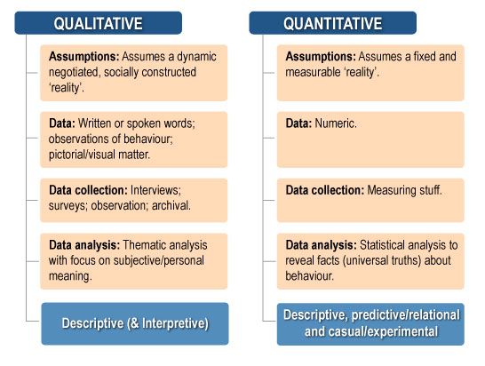
Quantitative approaches : These approaches use data with numerical values, counts or groupings assigned to them, measuring how many, how much, how often, how fast/slow and so on. Stated another way, quantitative data provide information about values or quantities, therefore, quantitative data can be counted, measured and expressed in numbers. Quantitative approaches assume a fixed and measurable reality. Data can be evaluated by making numerical comparisons and applying relevant mathematical and statistical procedures. Depending upon methodology and design, quantitative approaches have the capacity to describe phenomena, showcase relationships and, in some cases, establish evidence of cause and effect.

Qualitative approaches: These approaches do not have numerical values assigned, and the data are descriptive. Methodologically, qualitative data are grouped according to themes or like-minded descriptions (e.g. extracted from participant narratives such as opinions or views on things). Qualitative approaches are generally descriptive in nature and have no capacity to establish cause-and-effect relationships.

Qualitative approaches assume a dynamic, socially constructed reality. The approach involves collecting and analysing narrative, observational and pictorial data (e.g. from interviews, focus groups, open-ended surveys, archival footage and recordings). Thematic analysis is common in qualitative research. The analysis involves identifying ideas or groups of meanings. For example, assume a researcher is interested in the ‘felt experience’ of residents in an aged-care facility. By asking carefully selected questions to encourage resident elaboration on key topics (e.g. the propensity for engagement with other residents, thoughts as to the user-friendliness of the layout of the facility), the researcher can acquire a rich tapestry of information. By inputting this narrative information, thematic analysis might identify key recurring narrative themes. These ‘extractions’ subsequently form the basis of an interpretation and ultimately a report about what was identified. No numerical values are assigned to anything beyond simple counts of recurring themes and the percentages of people who expressed a particular view or thought.

In short, qualitative research is interpretive (i.e. the researcher attempts to understand data from the participants’ subjective experience) as opposed to data driven. Consequently, different researchers may derive different interpretations from the same data. Qualitative research is often undertaken in the field, such as within the context of an aged-care facility, so as to retain ‘naturalism’.

Also note that a mixed-methods approach might be used by some researchers, leveraging the advantages of both quantitative and qualitative methods to understand the subject better than any individual approach could offer on its own. Some researchers may also adopt an approach whereby they quantify qualitative data (e.g. assign numerical codes to themes or key words extracted from participant narratives, for use in quantitative analyses).

In this subject we deal almost exclusively with quantitative data and approaches. The term ‘statistics’ does not apply to qualitative data.

See the following figure for a summary of qualitative and quantitative approaches.

Variables in research

This topic provides an introduction to variables and their measurement properties.

Introduction

In this section we define a variety of common variables seen in research, and describe the type of measurement properties that might be assigned to them.

Variable types

Variable: These are characteristics or conditions that can assume more than one value (i.e. they can vary). In quantitative research, variables are assigned values, groupings or levels of some sort. Example variables include extraversion, intelligence quotient (IQ), age, gender, height, weight, self-esteem, perceived control and political orientation.

Variables are meant to represent some hypothetical construct or concept. A hypothetical construct is a theoretical concept that we operationalise (turn into a variable). In order to be accurately operationalised, the construct needs to be clearly defined as to what it represents and what it does not. An operational definition specifies exactly how we define and measure a variable. Note that a variable like IQ is really only an ‘alleged’ index of intelligence, unlike the operationalisation of the measurement of height.

To put it another way, variables are the operationalisation of constructs. Operationalisation is the procedure used to make the variables. An operational definition gets us started in this process by clearly defining what it is we want to measure and operationalise.

There are a variety of different types of variables based upon their construction and application. We now turn to discussion on these.

Dependent variable (DV): Also known as an outcome variable, response variable or criterion variable, the DV is assumed to be dependent upon the independent variable; therefore, change to the DV is the outcome being measured (e.g. reaction time, level of prejudice). A research design may include a number of DVs. The researcher does not interfere with or manipulate the DV, as it is meant to be impacted by the independent variable (IV).

Independent variable (IV): Also known as a predictor variable or explanatory variable, the IV is the variable assumed to influence the DV. A research design may include a number of IVs. Sometimes the IV is manipulated (e.g. prescribing different amounts of sleep to participants). In observational studies the IV is not manipulated.

Manipulated variable: The manipulated variable is a special type of IV. A manipulated variable in experimental research is an experimenter-imposed condition or grouping, or influence of some type (e.g. the researcher deprives one group of participants of sleep while the other group sleep normally and then they are all assessed on a reaction time task). Here the experimenter has manipulated the variable of sleep by allocating participants differing levels of sleep. Some variables cannot be manipulated such as IQ, physical injury or any action that may harm a participant.

Extraneous variable: This is a variable that is not an IV in the study but still influences the DV. The extraneous variable has a relationship (i.e. it is correlated) with both the IV and DV, but may not differ systematically with the IV. In reality, there are probably a great number of variables we do not measure or cannot measure and take into account that may have an impact on the DV. This is evident in research studies where we see a large amount of unmeasured or error variance in our statistical outcomes (which we will discuss later in the subject).

An extraneous variable might occur in the following way. A workplace study seeks to establish whether or not the addition of background music increases employee productivity in a packing plant based on the premise (hypothesis) that music will be motivating. The DV is the number of items packed in a given work shift. The IV comprises two levels: no music and music. Assume results show the average number of items packed by our employees to be greater in the music condition than the non-music condition. An extraneous variable might be another variable that accounts for the difference (e.g. the music induces a state of relaxation that enables performance instead of inducing a motivational state), so we have a third variable (the extraneous underlying variable accounting for the observed difference) instead of the hypothesised underlying variable. If we have not considered the potential influence of this third variable of relaxation in our design by, for example, measuring it, then we incorrectly assume employee motivation was influenced by music.

Confound variable: A confound is an extraneous variable that moves systematically with the IV (i.e. the mean value of the extraneous variable differs between IV levels) to influence the DV. Therefore, we do not know whether the IV, confound or both are impacting scores on the DV. Using our packing plant study example above (and assuming the same outcome difference), a confound might be introduced to the study if, for example, the workers in the music condition were those who worked later in the day, while those not exposed to music worked an earlier shift. There might be something about the time of shift that moves systematically with the IV (i.e. differs between the levels of the IV) such as level of concentration, tiredness, or perhaps age of employees who work later in the day versus earlier in the day. We do not know whether it was the IV, some aspect related to time of shift, or the influence of both that resulted in the observed outcomes.

As we can see, both an extraneous variable and a confound will muddy results interpretation because they impact DV scores. In other words, we cannot be sure the IV was solely responsible for changes in the DV when we have these additional variables as potential contributors to outcome differences. Note that it is the expectation that we cannot account for all potential extraneous variables. To have a dedicated confound in a design and not realise it (much more egregious) is embarrassing to a researcher! Also note that the terms extraneous variable and confound variable are often used interchangeably in research. In reality it can be quite difficult to distinguish between these types of variables.

There are two main ways to deal with suspected or known problematic variables.

• Create a design that excludes differential impact of unwanted variables. We can do this by holding procedures constant. For example, returning to our packing plant study, the time of shift could be held constant (i.e. test both conditions at the same time of day).

Some extraneous variables such as those involving individual differences among people (e.g. personality variables, IQ) can be ‘evened out’ through random allocation to conditions (e.g. drawing straws to allocate participants in the sample to treatment and control conditions). Although there are no guarantees, individual differences among people should now be fairly balanced between the conditions (only by chance occurrence should there be differences). These then are examples of designing problematic variables out of the study design.

• Include the problematic variable in the design. This is the approach to use when the problematic variable can be identified and measured. It is also the approach to use when the variable cannot be designed out of the study design, or when we actually want to know its effect. For example, let us assume we want to manipulate participants’ perceived personal control by creating a control loss state for half of our participants, and a control bolstering state for our remaining participants. The hypothesis is that control loss, in contrast to control bolstering, is more likely to motivate compensatory control-seeking behaviour (i.e. control loss is hypothesised to activate an attempt to restore the sense of lost control).

Therefore, we randomly allocate our participants (so that individual differences are largely balanced out) to either a low control condition or a high control condition (this is a between-subjects design, which means no participant is in both conditions). Our participants are then manipulated into a low control or high control state by recalling and writing about a time they had no control over an outcome or a time they had complete control over the outcome. This type of manipulation has been shown to invoke the relevant control states (Knight et al., 2014).

Let us assume for the moment that statistical analysis shows our hypothesis to be supported. Does this mean that relative levels of control were responsible for the outcomes? Perhaps not. It is possible that causing participants to think about a low control situation might make them feel bad (i.e. create negative affect), while those thinking about a high control situation may feel much better (i.e. they experience relatively less negative affect, if not positive affect). Thus, it may be that differences in affect or mood are impacting the outcomes alongside levels of control. Affect, then, is an example of a confounding variable in this design because it is expected to have both an influence on the DV and vary systematically with the IV of control.

As it is not possible to prevent such changes in affect (if they are there), the only option open to the researcher is to measure affect to determine or statistically control its impact. This is easily done with a scale that measures affect – the 20-item positive and negative affect scale (PANAS). Participants respond to PANAS items such as interested, distressed, upset and irritable based on how they are feeling right now. Participants use a scale from 1, very slightly or not at all, to 7, extremely. Note that we would measure affect very soon after participants complete the control manipulations so as to best see the potential effect of the manipulation tasks on affect. Now that affect is measured, we can assess its relative influence on the DV by factoring it in as another IV, or we can control for affect by averaging out the influence of affect across both the manipulated control conditions in our statistical analysis (more on control variables below).

Control variable: These can take a variety of forms. Some variables are controlled in that they can be held constant by the researcher. A control variable is often something that a researcher includes in a study that is not of key interest, but nevertheless should be measured and accounted for in analysis and results interpretation (it might be a well-considered extraneous variable or potential confound as we saw above). This then is a statistical control variable. For example, suppose a researcher is investigating the effect of different levels of sleep (IV) on a reaction time task (DV). If for some reason the researcher suspects that females might perform better under conditions of less sleep than males, but was not actually interested in this nuance (instead preferring to investigate the effect without regard to gender), gender could be statistically included as a control variable (i.e. the effects of gender could be averaged out across the conditions of eight hours’ sleep versus four hours’ sleep). Stated another way, this allows statistical interpretation of the effect of differing levels of sleep on reaction time after removing the differences in this relationship that are associated with gender. If, however, the researcher was actually interested in this gender difference, then gender might be included as a variable in the study in a more complex factorial design (i.e. two IVs: gender is one IV and sleep is another, with both IVs having two levels).

A general note: Control in research can mean different things.

1. A verification of an effect via comparison, such as using a control group in conjunction with a treatment group for the purposes of comparison
2. Restriction through holding aspects or variables constant, or to eliminate the influence of problematic variables, as in the control variable example above
3. Manipulating conditions so that their effects are both maximised and targeted, such as using a lab situation to generate greater control over the manipulations participants receive.

Person variable (PV) and person attribute variable (PAV): A PV is some aspect or difference tied to the participants, such as personality traits, attitudes, views, cognitive functioning, IQ, reading speed, employed/unemployed or male/female, that participants bring to the study (an individual difference).

A PAV is a person-variable put to use by the researcher as an IV in the design (e.g. the case of dividing participants into groups based on gender, with the purpose of exploring potential gender differences). Allocation to condition – levels of the IV – on the basis of a PAV means that full random assignment to condition is not possible. Not all PVs are PAVs, but all PAVs are PVs.

Manipulation check item: Manipulation check items are not technically variables, but have been included in this section given their variable-related focus. A manipulation check is included in designs where the researcher has manipulated the IV so as to determine whether or not the manipulation has worked. Manipulation checks take various forms, and may be as simple as subtly or indirectly asking participants what effect the manipulation had on them.

Returning to our study about feelings of control for a moment, we might include a question in the design, positioned after the manipulation, to get at participant perceptions of control. For example, we might ask participants to think back to the writing task and indicate how much control they had over the outcome they wrote about by recording their responses using the response format (1, absolutely no control, to 7, complete control). If we find that responses to this item correspond to the relevant manipulation the participant received, then we can assume the manipulation was at least sufficiently understood by the participant. This does not necessarily mean that the participants actually ‘internalised’ the manipulation, but it is about as close as we can get to ‘knowing’ whether or not the manipulation worked as intended. This outcome combined with the measurement and control of the potential confound of affect (explained earlier), provides us with a body of evidence that the study was internally valid (i.e. it was the desired manipulation that led to changes in DV scores).

Note, though, that the positioning of the manipulation check item is crucial to maintaining the integrity of the study. Positioning the check item immediately after the manipulation might illuminate the focus of the study to participants (i.e. the realisation it is about personal control). A manipulation check such as this is better positioned towards the end of the study, after the DV has been administered.

Variable measurement

In this section we look more deeply at the makeup of research variables and their measurement.

• Quantitative variables: These are variables expressed in some numerical fashion, and are classified as either ratio or interval variables.
• RATIO VARIABLES: have an absolute zero point and equal intervals, and assess magnitude (e.g. reaction time, height).
• INTERVAL VARIABLES: have no absolute zero point, but have equal intervals, and assess magnitude (e.g. degrees Celsius, IQ).
• Categorical variable: This is a variable with either natural or manipulated groupings, such as with/without depression, female/male, low/medium/high level of some attribute, low/high control state imposed by the experimenter. These variables are assumed to be discreet categories. A categorical variable can be either nominal (without rank order) or ordinal (with a rank order).
• Ordinal variables: Ordinal variables assess magnitude by virtue of being rank ordered, but have no set intervals or zero point (e.g. the ordering of a list of preferences or severity of illness ranked as mild, moderate and severe). Consider, for example, the finishing order of runners in a foot race. If we only look at the difference in finishing order, then this is an ordinal categorisation. The finishing order in this example tells us nothing about the distance or time interval between each finisher. However, the first runner over the line is assumed to have performed better than the second finisher, who has in turn performed better than the third finisher, and so on.
• Nominal variables: Nominal variables have no level of magnitude – no one category is seen to be more important than another (e.g. male/female, place of birth).

Note that the nature of any given variable and its scaling need to be considered when selecting a suitable statistical analysis. Measures of IQ, aptitude and personality are technically ordinal in nature. In many cases in psychology, however, such strictly ordinal measures are treated as though they are interval in nature because then we can justify the use of more powerful tests (i.e. those that potentially improve chances of finding important effects). This is because interval and ratio data are more open to statistical flexibility and manipulation, something we will explore with parametric and nonparametric tests later in the subject. For the moment, recognise that average scores (means) can be computed for interval and ratio data, but technically not for ordinal or nominal data.

Describing data patterns

This topic introduces ways by which collections of data might be summarised and understood.

Introduction

Collections of data form patterns that can be understood in terms of measurement of central tendency (how data are grouped around some central value) as well as in terms of spread and dispersion. We look to these and related concepts in this topic.

Introduction to the normal curve

The arrangement of the values of a variable is called the distribution of the variable. The normal curve/distribution (also known as the bell curve or the Gaussian distribution) reflects the notion that many continuous data in nature display a bell curve when graphed. The normal distribution is the most useful distribution in statistics, as most datasets can be approximated normally, and nearly all sampling distributions eventually converge to a normal distribution.

For example, if we sample a number of people who are representative of the population and we measure attributes such as IQ, height, weight, personality, driving ability or athletic prowess, we would see a curve emerge as we plot all those values. The midpoint reflects the point where most people’s scores will reside (e.g. the average). If, for example, we have plotted scores for athletic ability in such a way that higher scores reflecting greater athletic ability are to the right of the midpoint of the distribution, then we can see that as scores increase, the number of people who are so gifted decreases. Similarly, those persons who are less gifted will be seen in the tail of the left side of the distribution.

These are the core properties of a normal distribution:

• The mean, mode and median are all equal.
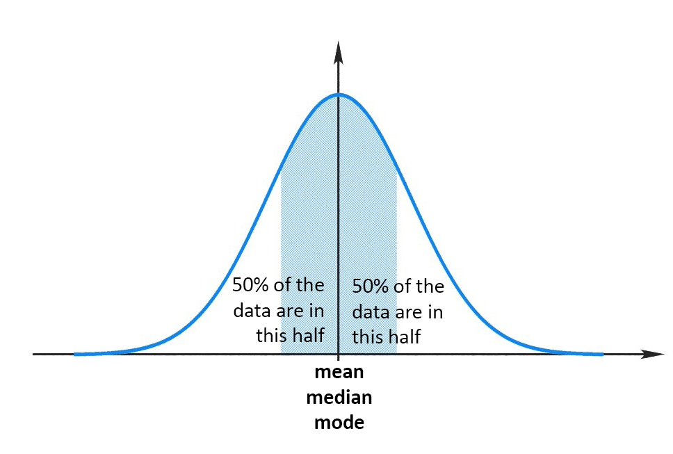
• The curve is symmetrical with half the values lying to the left of the centre and half to the right of the centre.
• The total area under the curve is 100 per cent, expressed as 1.

See Figure 1.4.1 below depicting a normal distribution of scores. Note that it is symmetrical, and the mean (i.e. the average score), median (i.e. the middle score) and mode (i.e. the single most frequent score) all sit on top of one another (i.e. they are equal).

Note that score distributions can reflect different things (e.g. percentages, frequencies). A distribution of percentages of a group of people in different age groups is a percentage distribution of age. If the actual numbers or frequencies in these age groups are presented instead of percentages, we have a frequency distribution. Distributions can also be referred to as probability distributions when making likelihood assessments. For example, scores closer to the tail ends of a normal distribution are less likely to be predictive of the mean, median or mode. Therefore, a probability distribution shows the chance, or probability, that the value of a variable will lie in different areas within its range.

We will revisit the normal distribution (bell curve) in more depth a bit later when we discuss standard deviation and Z-scores. For now we turn to measures of central tendency (i.e. mean, median and mode) and variability so as to better understand the properties of distributions.

Measures of central tendency

A measure of central tendency is a descriptive statistic indicating the average or mid-most score between the extreme scores in a distribution of scores. Depending on distribution shape, the mean, median or mode may be the best measure of central tendency. These are three main measures of central tendency (how scores tend to cluster in distributions of scores).

Mode: This is simply the most frequently occurring score in a given frequency distribution. There may be more than one mode in a given distribution of scores if two or more scores recur at the same frequency. The mode best caters to nominal data. Note that because of its peculiarities, the mode may not actually be a measure of central tendency at all (i.e. if the most frequent occurring score is nowhere near the middle of the distribution).

Median: When all scores in a given distribution of scores are arranged from lowest to highest, the median is the score positioned in the middle. Stated another way, the median score splits the distribution of scores in two, such that there are the same number of scores above and below the median score. Whenever there is an odd number of scores, the median is the middle number. Whenever there is an even number of scores, the median is the average of the two centremost numbers. The median is useful for ordinal, interval and ratio data. The median is particularly useful when the distribution is highly skewed (i.e. when scores truncate at either the upper or lower end of a distribution of scores). The median remains unaffected by the highest and lowest scores.

Mean: The mean is the average of any summed scores – the sum of the scores divided by the number of scores. The mean has unique properties in statistics given that it is the value upon which variability is calculated (i.e. the variance and standard deviation, but more on these later). The mean is usually the most appropriate measure of central tendency in a normal distribution of scores involving either interval or ratio data. As psychological researchers, we find the mean is usually the most useful measure of central tendency and thus calculate mean scores for grouped data.

Unlike both the mode and median, though, the mean is sensitive to every other score in the distribution. Consequently, even a small number of particularly high or low scores provided by a participant or participants can ‘skew’ or change the shape of the overall score distribution quite considerably. That is, extreme scores tend to drag the mean value towards them. Also, a small number of the same extreme scores in a relatively small sample will have a stronger influence on the mean.

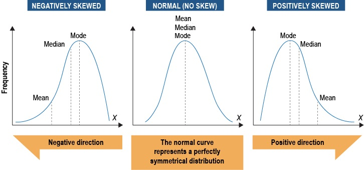
We saw earlier how the mean, median and mode are all equal in a normal distribution. But things change considerably when we do not have a normal distribution of scores – when the distribution is skewed. The mean is affected the most by outlier values (i.e. unusual or deviant values in the distribution compared to the other values), which may be especially small or large in numerical value. The mean is pulled in the direction of the skew. So when the distribution departs from normality in a negative direction, the mean is now less than the median, which is less than the mode. When the distribution is positively skewed, the mode is greater than the median, which is greater than the mean. When the distribution is skewed it might be better to use the median instead of the mean because it is not influenced by extreme scores.

Depicting the normal distribution and positively and negatively skewed distributions below.

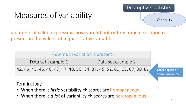
Measures of variability

While measures of central tendency tell us what is typical for a variable, variability tells us how spread out the scores are. Measures or expressions of variability include the range, interquartile and semi-interquartile range, the variance, and the standard deviation (SD). There are other measures of variability as well, but the main ones we cover in this subject are the different types of ranges, variance and SD. The three measures of central tendency we looked at earlier (the mode, median and mean) are single numbers that provide information about the central tendency of the score distribution (although the mode is not always a measure of central tendency). But just as important are ways to quantify how spread out (dispersed or variable) the scores that make up the distribution are.

To put it as simply as possible, if all our collected scores were found to be the same, there would be no variability. The more different the values collected are, the more variability there is. See Figure 1.4.3 below identifying greater variability among scores in dataset example 2.

Range: The range is the difference between the lowest score and the highest score – the largest value minus the smallest value. Assume we have a scale with a possible scoring range of 1 to 50. Participants’ responses, though, may not fully encompass the possible range. For example, perhaps no one in our sample scores higher than 40 on the scale. So we have both a possible or theoretical response range, and the actual range (in terms of data) that participants supply.

The range is limited in that it only provides information about the lowest and highest scores obtained in a sample; it provides no indication of variability among the rest of the scores. For example, assume that of 50 responses made on a scale from 1–100, all but one response is between the values of 10 and 50, while the one remaining response is 99. Here we have a single extreme score (an outlier), while most of the remaining variability is much lower in the scale range. Therefore, this spread is not a particularly good indicator of the actual variability existing among scores, but rather just indicates the breadth. This is not to say that this extreme score is not important; at the very least we would like to know how it came about when everyone else is scoring much lower (i.e. is it a true extreme score, a mistake/error, or due to chance?).

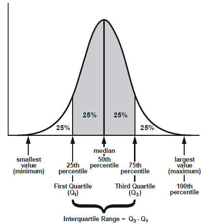
Interquartile and semi-interquartile ranges: A distribution of scores can be divided into four parts so that 25 per cent of scores end up in each quarter. The term ‘quartile’ refers to a point, while the term ‘quarter’ refers to an interval (or band). The second quartile is, therefore, the median score (positioned at the 50th percentile). The interquartile range is a measure of variability equal to the difference between quartiles one and three. The semi-interquartile range is the quartile range divided by two. See Figure 1.4.4 below displaying the interquartile range.

We now turn to the variance and SD because, unlike the range, they take into account all values in a given dataset.

The variance: Variance can be a difficult concept to understand given that it can take a number of forms. To complicate things further, sometimes (depending on context) we want variance and sometimes we do not. As researchers, we often want to see some variability in our data, as long as it is ‘good’ variability. We, however, do not want to see variability from ‘error’ or unmeasured variance (but more on this later in the subject and the other contexts where we actually might want to minimise variability).

Variability in a questionnaire, for example, means that people are responding differently (we expect to see differences among people in terms of their attitudes and beliefs). If we had little to no variance among our participants responses then we would have to assume either: (a) we have selected a homogenous sample of participants in terms of their views (i.e. they truly do not vary much); or (b) the questionnaire lacks measurement sensitivity (i.e. the scale items cannot generate variability, perhaps because items are poorly worded or are too much alike).

Formally, the variance is a single value that is the mean of the squared deviation scores. Practically, it is the mathematically squared extent to which scores in a given distribution differ both from the mean and one another. Stated another way, the variance represents the size of differences from one mean score to another. It is popular because it has nice mathematical properties.

To calculate variance (no, you will not have to calculate variance):

1. Subtract the mean from each value in data. This provides a measure of the distance of each value from the mean.
2. Square each of these distances (so that they are all positive values), and add all of the squares together.
3. Divide the sum of the squares by the number of values in the dataset

σ2=∑(χ−μ)2N

Where:

• σ2σ2= variance
• ∑∑ = the sum of
• χχ = score/value
• μμ = mean of the population
• NN = number of values

The variance has some interesting properties. If all scores in a given distribution are quite similar then the variance among scores is small. As scores vary more, the variance increases. Consequently, it is possible to have more variance in a distribution with a small number of scores than in a distribution with a larger number of scores, assuming of course, the score values differ more in the smaller distribution of scores.

Standard deviation (SD) ; The standard deviation is the measure of variability we will encounter most often in this subject. This is because the SD is a fundamental part of the reporting of statistical outcomes, and it is conceptually easier to interpret than the variance given the values it provides. In other words, the SD turns the variance into more meaningful units which help in interpretation. Mathematically, it is simply the square root of the variance. Therefore, the variance is the standard deviation squared. The SD reflects standardisation of the score distribution. What this means is that the mean of the distribution is now converted to zero with a SD of one (unlike the variance). The SD tells us the average distance our data values are from the mean in standard units. Note that standardising the normal distribution in this way does not change the shape of the distribution. You will not be asked to calculate a standard deviation.

Standard deviation: σ=√σ2σ=σ2

Or

σ=√∑(χ−μ)2N

In a nutshell, both the variance and SD are interpreted in the same way. Larger values indicate greater variation among the scores, while smaller values indicate less variation among the scores. The SD, however, is more easily interpreted than the variance, as we will see shortly (i.e. the units of variability provided by the SD is conceptually easier to relate to the distribution values ).

SD and the normal distribution

We have determined that a normal distribution is a mathematically derived theoretical distribution, which is symmetrically shaped. The mean, median, and mode are all equal in such a distribution. For a quick primer on what is to follow, see the video below.

• StatQuest with Josh Starmer. (2017). StatQuest: The Normal Distribution, Clearly Explained!!!. YouTube.

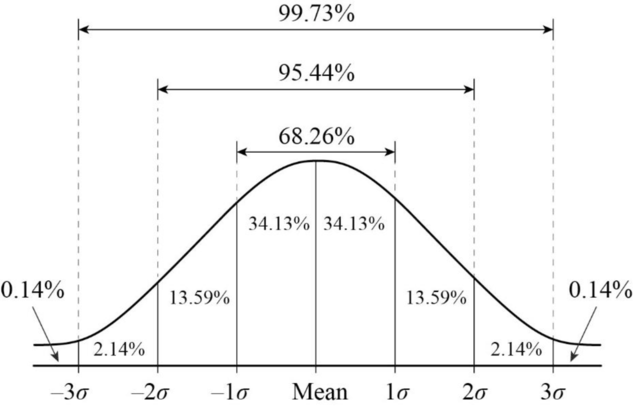
In a normal distribution, 68.26 per cent (68 per cent) of all observations/scores lie within one standard deviation either side of the population mean, while 95.44 per cent (95 per cent) of all observations/scores lie within two standard deviations either side of the population mean. Similarly, 99.73 per cent (97 per cent) of all observations lie within three standard deviations either side of the population mean. This division is known as the 68-95-99.7 rule. Recall that the mean and SD can be calculated for a dataset. The mean is the value by which the variance and SD are calculated. By knowing the SD (i.e. the standardised variance) we have a ‘standard’ way of conceptualising how extreme scores in a distribution of scores may be. Indeed, often in statistics we refer to data in terms of SD. See figure of the normal distribution that also depicts SD points (symbol σσ).

Watch the video below for an intuitive introduction to the application of the SD in probability terms.

• Jeremy Jones. (2015). Standard Deviation – Explained and Visualized. YouTube.

See this video for further elaboration, as well as how to go about calculating the SD. (Warning: exposure to math, but in a good user friendly way. Highly recommended

• Jeremy Jones. (2016). How to Calculate Standard Deviation. YouTube.

View the following video for a summary on the normal distribution and areas under the curve.

• Simple Learning Pro. (2019). The Normal Distribution and the 68-95-99.7 Rule (5.2). YouTube.

Z-scores

Z-scores are raw scores that has been transformed into SD units. Therefore, Z-scores are raw scores converted into a standardised metric such that the mean is now zero and the SD is one. What this standardisation does is that it allows for interpretation of data values in terms of how far they might be from the mean of the distribution. The math formula for turning a raw score into a Z-score is quite easy to understand and calculate (the mean is subtracted from a given raw score value, then this figure is divided by the SD.

Why might Z-scores be useful? One useful application is when we want to compare scores from different distributions that have different means and SDs. For example, suppose that a student takes two tests: A test on introductory statistics, and a test on math. Both are marked out of 100. Our student scores 65 on statistics, and 75 on math. When comparing relative performance on the tests we might offer up the conclusion that our student did relatively better on the math test than the statistics test. But we best look to the means (for all students) on each test before locking in this conclusion. Assume the mean score for the statistics test was 50 while the mean score for the math test was 60. Now in which test did our student do better? It looks like a tie given that our student is 15 points higher than the mean on both tests (i.e., the student’s deviation from the mean is the same for both tests). Assume that the SD for the statistics test is 10, while the SD for the math test is 15. Based on SD units from the mean we can now see that our student is 1.5 SDs above the mean on the statistics test, but only one SD above the mean on the math test. So relatively speaking, our observed test-taker has done better in statistics than in math. In other words, our student is further along the distribution in relation to the other test-takers when it comes to statistics than math. How was this standardised relevance achieved? Z-scores always have a mean of 0 and SD of 1. By converting different distributions to Z-scores we can now directly compare them (because they each have an identical mean and SD).

Z-scores are also particularly useful when participants are being measured on scales that use different response formats. For example, it might be problematic to compare means across scales ostensibly measuring the same construct, but which have different response formats.

For example, assume we have two measures of self-reported life satisfaction, one was used on one sample and the other measure was used on a second sample. If one measure though used the following response format (1 = strongly disagree to 7 = strongly agree), while the other used the following response format (1 = strongly disagree to 5 = strongly agree) we cannot directly compare them (i.e. the scaling is different). By converting our raw scores for each scale to Z-scores (with a mean of 0 and SD of 1), they can now be compared.

In order to cement your understanding of the standard distribution and Z-scores, see the following video. One of the examples in the video relates to American college admission tests, but the video illuminates key points in a recipient friendly manner regardless.

• CrashCourse. (2018). Z-Scores and Percentiles: Crash Course Statistics #18. YouTube.

Data collection methods

This topic presents common data collection methods used in psychological research.

Introduction

Data collection refers to how researchers (and others) go about obtaining data. Before we can analyse data, we need to collect them, and there are a number of methods or ways to go about collecting data. There are various typologies used to explain and differentiate these methods. In this subject we focus on a typology involving six general data collection methods:

• Tests (e.g. of personality, mental health status, cognitive capacity)
• Questionnaires/surveys (e.g. beliefs, attitudes)
• Interviews
• Focus groups
• Observations
• Existing data.

Data collection methods

TEST: Tests can be any assessment of personality, mental health status, cognitive capacity, achievement, skills or behaviours administered in some way. Such tests may involve complex scanning equipment, or at the other end of the continuum, simple administration via paper and pencil. We can broadly classify these types of tests as either standardised or researcher constructed.

For example, tests of IQ are standardised in terms of having been thoroughly tested on the specific populations (i.e. children versus adults) for which they are focussed. There are norms of population performance that have been established, and such standardised tests have been shown to be valid and reliable. Standardised tests, therefore, have a body of support for their utility, so they should be the first point of call for a researcher looking for an instrument to measure IQ or some other construct for which standardised assessment tools are available. Many standardised tests of personality can usually be found by undertaking a literature search; while some clinical measures and those with proprietary rights attached may only be available from resource libraries or manufacturers, and are hidden behind paywalls.

The other approach is for the researcher to create their own test. This is appropriate when measuring a nuanced construct, when a standardised test is not available, when attempting to improve upon an existing test or when developing a new instrument (e.g. a new scale).

Questionnaires/surveys: These are self-report measures often used to collect data on opinions, views, attitudes and the like. At the most fundamental level, surveys may comprise either open-ended questions or closed-ended questions (often called items). Open-ended questions allow participants to respond and elaborate using their own words, lending more to qualitative research, while closed-ended items only allow a participant to choose from provided options (often referred to as forced-choice surveys).

Closed-ended items are numerically coded for use in quantitative analysis. The survey respondent is said to have more or less of what is being measured as judged by their test score. Closed-ended items are much easier to analyse in comparison to open-ended questions by virtue of their not needing to be read and coded.

The response format on forced-choice surveys and questionnaires can vary considerably among instruments. Scaling refers to the way numbers or indices are assigned to different amounts of what is being measured. Example response formats include the following.

Dichotomous scale: A dichotomous scale provides two options:

• Yes/no
• True/false
• Agree/disagree.

An example item: ‘Have you ever stolen something from a store?’

Response options: Yes/no

Note that a dichotomous response format provides nominal data.

Likert scale: A summative scale usually comprising 5, 7 or 9 response options, and a number of items. The participant responds to a set of statements (items) by rating level of agreement with those statements. The most common Likert format has anchor labels ranging from strongly disagree to strongly agree so as to assess attitudes.

An example item: ‘Stealing from a store is never justified.’

Response options: 1 = strongly disagree to 7 = strongly agree

Note that a Likert format provides ordinal data.

Rating scale: Rating scales comprise ordered numerical or verbal descriptors on a continuum upon which judgements can be recorded.

Example item: ‘How much did you enjoy this meal?’

Response options: 1 = not at all to 10 = very much

Note that this format provides ordinal data.

Paired comparison scale: Test-takers are presented with pairs of stimuli (e.g. photos, statements, objects) and are asked which they prefer.

An example item: ‘Select the behaviour you think is more justified.’

Response options:

1. Cheating on taxes
2. Accepting a bribe

Note that this format provides ordinal data.

Guttmann scale: This is a format where a series of statements range sequentially from weaker to stronger in terms of the belief or attitude being measured. A feature is that the respondents agreeing with the stronger statements should also agree with the milder statements.

Example item: ‘Do you agree or disagree with each of the following?’

Items:

1. All people should have the right to suicide (the most extreme position).
2. People in pain or who are terminally ill should have the option of assisted suicide.
3. People should have the right to refuse life support systems.
4. People have the right to be comfortable in life (the least extreme position).

Response options: Agree/disagree

Note that this format provides ordinal data.

Semantic differential scale: These scales usually have words with polar-opposite adjectives at each end of a rating scale. The scale format is often used to assess participant beliefs.

An example item: ‘When thinking about [insert computer brand and model], how would you rate it on the following attributes?’

Response options:

• 1 = Innovative to 5 = Dull
• 1 = Inexpensive to 5 = Expensive.

Note that this format provides ordinal data.

These are just some examples of various rating and response formats. Also note that it is not uncommon for definitions to vary across texts and resources (e.g. some purists may argue that a Likert scale evaluates agreement only, and should only have five response options).

Visit the Qualtrics website (a survey building resource and data acquisition service often used by academics) for further information on response options and scale formats.

Interview: This is a data collection method in which the interviewer asks questions directly, although this can be face-face, by phone, video conference or email. The questions may be open-ended or closed. Interview formats using open-ended questioning are often used in qualitative research so as to encourage rich elaboration. Face-to-face and phone interview formats are examples of synchronous interaction (i.e. in real time), while email interviews are an example of asynchronous interaction (i.e. exchanges take place over time).

Interviews range from being highly structured (providing a set of specific prepared and ordered questions) to unstructured (providing a general list of topics to explore).

Focus groups: Focus groups comprise a small number of participants (generally 6–12) convened by a researcher to explore how people in a community might think about an issue (e.g. the handover of a green space to property developers). The idea is to glean information about common perceptions and beliefs from those potentially most affected (i.e. those who might benefit and those who might suffer). Focus groups are a feature of qualitative data collection, but are sometimes used in quantitative research to gain a better understanding of participant perceptions, understanding and concerns, in order to facilitate and refine quantitative research options (e.g. to allow the development of targeted surveys, to identify key themes that point to specific variable inclusion).

With focus group data acquisition, the convener/researcher provides the topics and moderates the discussion. A key role of the moderator is to keep discussion on topic while also allowing prudent tangents to be pursued.

Observations: A key focus of direct observation is to uncover what people actually do as opposed to what they say they do. However, there may be reactive effects (i.e. atypical behaviour) when participants know they are being observed.

Quantitative-based observational data may be collected openly or surreptitiously depending on the aim. Naturalistic observations are those conducted in the real world (e.g. observing behavioural tendencies such as physical distancing from others within or across natural settings). Observations undertaken in laboratory settings are potentially more manifest to participants, unless participants have been provided with a cover story to hide the true nature of the observations being undertaken. For example, female participants might be brought into a lab under the pretence of completing a survey, yet unbeknownst to them the real focus is on observing their behaviour when interacting with a male versus female researcher of varying levels of approachability and attractiveness. The degree of eye contact, physical distancing, as well as subtle and more overt flirtation might be recorded and coded for the purposes of quantitative analysis.

Some behavioural observations can be somewhat subjective (as in the above example) unless clearly operationalised in terms of exactly what comprises a given behaviour, including who, what, where, when, and how. Behavioural frequency and duration may also be important considerations. Checklists and the standardisation of observational measurement are important in ensuring consistency among observers/data recorders.

Where continual observation is not required, a time-interval approach may be used (e.g. making observations at pre-determined time intervals).

Within observation research, the relationship between the observer and the subject can be important. There are four ways to categorise this relationship.

Existing Data: In this era of ‘erase no data’ and ‘sell off others’ data’ the opportunity to use existing or previously acquired data is growing. Often existing data are picked up by researchers for a purpose other than that for which they are being currently used. Existing data are by definition retrospective, and may be used in retrospective longitudinal designs.

Sources of existing data include:

• Personal documents (e.g. letters, diaries, photos)
• Official (e.g. written and recorded public and private documents such as meeting minutes, annual reports, newspapers)
• Physical data (e.g. DNA, trash, trace elements)
• Archived research data (e.g. repository data, government health and planning data)
• Anything you put into a Google search!