Introduction
Regression analysis is a statistical tool that is used to develop approximate linear relationships among various variables. Regression analysis formulates an association between several variables. When coming up with the model, it is necessary to separate between dependent and independent variables. Regression models are used to predict trends of future variables. The paper carries out both simple and multiple regression analyses of the Keynesian consumption function. Consumption is a function of income and wealth. Consumption from a sample of 25 households is used in the analysis.
Scatter diagram
A scatter diagram is a graph that plots two related variables on a Cartesian plane. The independent variable is plotted on the x-axis while the dependent variable is on the y – axis. In this case, the amount of consumption is plotted on the y – axis while the wealth and annual disposable income are plotted on the x-axis. Different graphs will be plotted for each explanatory variable. A Scatter diagram tries to establish if there exists a linear relationship between two variables plotted on the diagram. This can be observed by looking at the trend of the scatter plots. The graph below shows the scatter diagram of consumer expenditure (Y) against disposable income (X1).
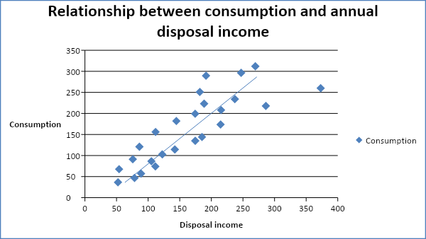
The scatter plots on the diagram above tend to slope upwards. The points on the diagram tend to concentrate along the line. This indicates a strong positive relationship between the variable. The correlation coefficient shows the value of correlation between consumption expenditure and annual disposable income.
The graph below shows the scatter diagram of consumer expenditure (Y) against the level of wealth (X2).
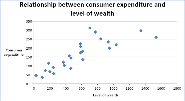
The scatter plots on the diagram above tend to slope upwards. This indicates a strong positive relationship between the variable. Thus, it is clear that both variables have a positive relationship with consumer expenditure.
Regression of total consumer expenditure on annual disposal income
The dependent variable is the total consumer expenditure while the independent variable is the amount of annual disposable income. A sample of twenty-five households is used to estimate the regression equation.
The regression line will take the form.

when the ordinary least squares method is used. The regression line can be simplified as shown below.
Simplified regression equation Y = b0 + b1X1
Y = Consumer expenditure
X1 = annual disposable income
The theoretical expectations are b0 can take any value and b1 > 0.
Regression Results
From the above table, the regression equation can be written as Y = 0.969973X1. The coefficient value of 0.969973 implies that as the annual disposal income increases by one unit, the consumer expenditure will increase by 0.969973 units. The positive value of the coefficient implies a positive relationship between the consumer expenditure and annual disposal income as was evident in the scatter diagram. The regression line can be drawn on the scatter diagram as shown below.
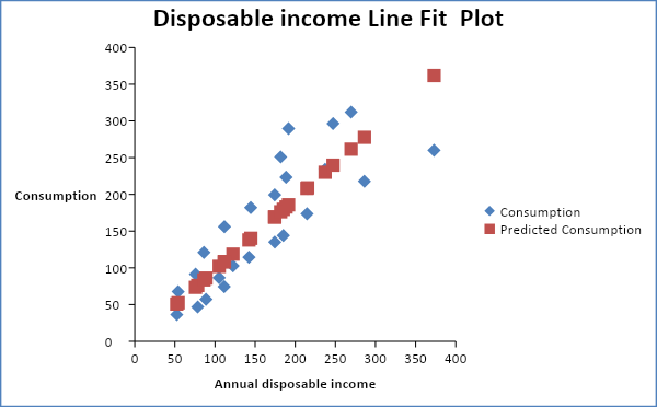
In the above diagram, the line of best fit is shown by the plots of predicted consumption.
Evaluation of regression model
Evaluation of the regression model can be done by testing the statistical significance of the variables. Testing statistical significance shows whether the annual disposal income is a significant determinant of the total consumer expenditure. A t-test will be used since the sample size is small. A two-tailed t-test is carried out at a 95% level of confidence.
Null hypothesis: Ho: bi = 0
Alternative hypotheses: Ho: bi ≠ 0
The null hypothesis implies that the variables are not significant determinants of demand. The alternative hypothesis implies that variables are a significant determinant of demand. The table below summarizes the results of the t-tests.
From the table above, the values of t – calculated are greater than the values of t – tabulated. Therefore, the null hypothesis will be rejected and this implies that the annual disposable income is a significant determinant explanatory variable. Thus, annual disposable income is statistically significant at the 95% level of significance.
R-square value
Coefficient of determination estimates the number of variations of the dependent variable explained by the independent variables. A high coefficient of determination implies that the explanatory variables adequately explain variations in the demand function. A low value of the coefficient of determination implies that the explanatory variables do not explain the variations in consumer expenditure adequately. For this regression, the value of R2 is 93.72%. This implies that the annual disposable income explains 93.72% of the variation in consumer expenditure. It is an indication of a strong explanatory variable. Also, the value of adjusted R2 is high at 89.56%. The value of R2 can be improved by adding more variables to the regression model.
Analysis of variance
The ESS is greater than RSS by a large margin. From the table, the explained sum of squares (93.72%) is equal to the value of R2 discussed above. It shows that the model is relevant in determining the variations in consumer expenditure. This is consistent with the real-life situation where the consumption of people highly depends on disposable income.
Regression of total consumer expenditure on level of wealth
The dependent variable is the total consumer expenditure while the independent variable is the level of wealth.
The regression line will take the form

when the ordinary least squares method is used. The regression line can be simplified as shown below.
Simplified regression equation Y = b0 + b2X2
Y = Consumer expenditure
X2 = level of wealth
The theoretical expectations are b0 can take any value and b2 > 0.
Regression Results
From the above table, the regression equation can be written as Y = 0.254056X2. The coefficient value of 0.254056 implies that as the level of wealth increases by one unit, the consumer expenditure will increase by 0.254056 units. The positive value of the coefficient implies a positive relationship between the consumer expenditure and the level of wealth as was evident in the scatter diagram. The regression line can be drawn on the scatter diagram as shown below.
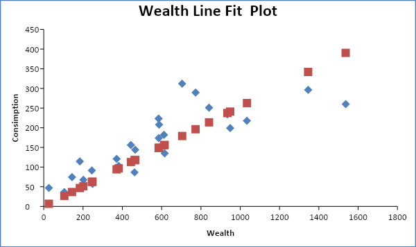
In the above diagram, the line of best fit is shown by the plots of predicted consumption that tend to take a straight line.
Evaluation of regression model
A two-tailed t-test is carried out at a 95% level of confidence.
Null hypothesis: Ho: bi = 0
Alternative hypotheses: Ho: bi ≠ 0
From the table above, the values of t – calculated are greater than the values of t – tabulated. Therefore, the null hypothesis will be rejected and this implies that the level of wealth is a significant determinant explanatory variable. Thus, the level of wealth is statistically significant at the 95% level of significance. The regression model shows that the slope is strong and the regression coefficient shows a positive relationship between the consumer expenditure and level of income.
R-square value
The value of R2 is 91.04%. This implies that the level of wealth explains only 91.04% of the variation in consumer expenditure. It is an indication of a strong explanatory variable. Also, the value of adjusted R2 is high at 86.87%.
Analysis of variance
The ESS is greater than RSS by a large margin. From the table, the explained sum of squares (91.04%) is equal to the value of R2 discussed above. It shows that the model is relevant in determining the variations in consumer expenditure. This is consistent with the life income hypothesis theory.
Prediction
Using the regression line Y = 0.969973X1, the values of consumer expenditure can be predicted as below.
Multiple regression analysis
Regression of total consumer expenditure on disposable income and level of wealth
The dependent variable is the total consumer expenditure while the independent variables are disposable income and the level of wealth. The regression line will attempt to establish a linear relationship between consumer expenditure, disposable income, and level of wealth.
The regression line will take the form

when the ordinary least squares method is used. The regression line can be simplified as shown below.
Simplified regression equation Y = b0 + b1X1 + b2X2
Y = Consumer expenditure
X1 = Disposable income
X2 = level of wealth
The theoretical expectations are b0 can take any value and b1, b2 > 0.
Regression Results
The result of regression for each independent variable is shown in the table below.
From the above table, the regression equation can be written as Y = 0.677219X1 + 0.080833X2. The intercept value of 0 implies that the line of best fit originates from the origin. The coefficient values are positive, that is, there is a positive relationship between disposable income and wealth. The values of the coefficient of both disposal income and wealth are lower than the values of multiple regression analysis. This can be as a result of some element of relationship with the explanatory variables.
Evaluation of regression model
Testing statistical significance shows whether the level of wealth is a significant determinant of the total consumer expenditure. A two-tailed t-test is carried out at a 95% level of confidence.
Null hypothesis: Ho: bi = 0
Alternative hypotheses: Ho: bi ≠ 0
The null hypothesis implies that the variables are not significant determinants of demand. The alternative hypothesis implies that variables are a significant determinants of demand. The table below summarizes the results of the t-tests.
From the table above, the value of t – calculated for annual disposable income is greater than the values of t – tabulated. Therefore, the null hypothesis will be rejected and this implies that the annual disposable income is a significant determinant explanatory variable. However, the level of wealth is not statistically significant since the null hypothesis will not be rejected. Thus, it can be dropped in the regression model. Besides, there is a high likelihood that the level of wealth is highly related to the disposal income since wealth is generated from disposal income among other factors.
R-square value
The value of multiple R is 97.16%. The value of R2 is 94.40%. This implies that the variables explain only 94.40% of the variation in consumer expenditure. It is an indication of a strong explanatory variable. The value is higher than those of the individual values since more variables improve on the value of the coefficient of determination.
Analysis of variance
The table below summarizes the analysis of variance.
The ESS is greater than RSS by a large margin. From the table, the explained sum of squares (94.40%) is equal to the value of R2 discussed above. It is worth noting that the increasing number of variables increases the value of ESS.
Prediction
Using the regression line Y = 0.969973X1, the values of consumer expenditure can be predicted as below.
Descriptive statistics
The table below summarizes the descriptive statistics of some variables.
Regression model
The regression model is given by the equation below.

The results of the regression are summarized in the table below.
The regression equation can be written as Y = -1256.764 + 0.2909rgdpch1970 +1426.6415avgsch1970 + 63.08lifeex1970 + 26.85trade1970. All the coefficients are positive. This implies that they contribute positively to real GDP per capita in 2005. A two-tailed t-test is carried out at a 95% level of confidence.
Null hypothesis: Ho: bi = 0
Alternative hypotheses: Ho: bi ≠ 0
Since the null hypothesis is rejected for all the coefficients of explanatory variables, it implies that all the variables are statistically significant.
Estimating the equations using the log of variables
The results of the regression are summarized in the table below.
The regression equation can be written as Y = 1.95 + 0.39rgdpch1970 +1.02avgsch1970 + 0.87lifeex1970 – 0.49trade1970. All the coefficients are positive apart from trade. Besides, their values are reduced. All the variables are statistically significant apart from trade for 1970 at the 95% level of confidence.
Correlation matrix
The table below summarizes the correlation matrix.
There is slightly a high correlation between the average schooling in 1970 and real GDP per capita in 2005. All the other correlation coefficients are low. Thus, there is no collinearity between the variables in the regression equation above. Multicollinearity is a condition when the explanatory variables are strongly correlated. Some of the other elements that need to be observed are high values of standard error and low values of the t – ratio. These are not found in the regression above and thus, multicollinearity does not exist in the above regression.
Test for autocorrelation
Autocorrelation is a scenario where the error terms of different periods are related. It is often tested either graphically or by use of the Durbin Watson test. The residual plot will be observed to ascertain if autocorrelation exists.
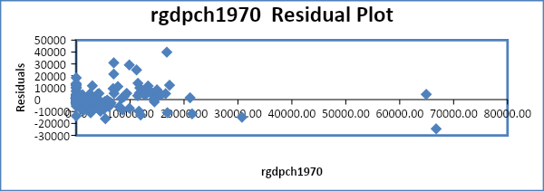
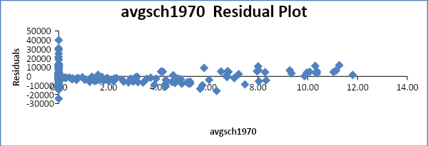
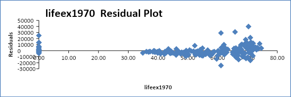
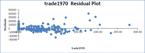
From the residual plots above, it is evident that there is no autocorrelation in most of the variables.
Robust standard errors or Whites heteroscedasticity correlated standard errors
Heteroscedasticity is a scenario where the error term violates the assumption of constant variance. The standard error of the regression equation is 7510.717929. The standard errors which arise when there is heteroscedasticity are known as robust standard errors. Generally, the standard errors shown above are not correct since the robust standard errors are more than the standard errors generated from the regression analysis. This gives an indication of the possible existence of heteroscedasticity. In the regression above, the robust standard errors are 8010.92728. It is an indication of the possible existence of heteroscedasticity.
Estimation of the average GDP per capita of Western Europe
The data of Western Europe is regarded as a dummy variable. Thus, it is important to use the various ways of carrying out regression using dummy variables. A dummy variable is regarded as a binary variable that takes the value either zero or one. Panel data analysis or random-effects models are used to analyze the regression equation. There will be a need to include two additional variables for the dummy variable that is dieurope0 and dieurope1. Thus, the regression equation will take the form shown below.

The table below summarizes the results of the regression with the dummy variables.
From the table above, it is clear the dummy variable westerneurope1 has a positive slope. In addition, it is statistically significant. There are a number of ways by which the regression model can be improved. One way is by lagging the dummy variables by one or two years. This will help in improving the efficiency of the model.