Arm Span vs. Height: The Relationship Analysis

Topic: Relationship Words: 2309 Pages: 8

Introduction

Vitruvius was a Roman architect and engineer who existed in the first century B.C. He used a formula to describe what he considered to be ideal male dimensions. Leonardo da Vinci, a famous Italian Medieval innovator and painter was influenced by this work. In 1490, Da Vinci used Vitruvius to draw a model that he referred to as Vitruvian Man (Alzyoud et al., 2021). A guy stands in a square inside the circle in Da Vinci’s artwork. The man has two sets of legs and arms outstretched. This study will demonstrate whether the men’s spread arms are equal to their height using the dimensions provided in the Vitruvian man illustration.

Da Vinci’s concept of the Vitruvian man and its proportion is fascinating. Due to this, it has formed the basis of the present study of wanting to see if there is a substantial correlation between height and arm span (Cadelano et al., 2020). Additionally, the study seeks to determine if height can be represented by arm span. If the study proves that arm span can represent the height, it can be used for clinical purposes when a patient cannot stand upright. To conduct the study, the hypothesis is:

Null hypothesis (H₀): Arm span and height do not have a significant positive association.
Alternative hypothesis (H₁): Arm span and height have a significant positive association.

Considerations

In this study, a sample of 100 students was selected from census-at-school data as participants. The sample contained both male and female genders, and the youngest student was 7 years while the oldest was 19 years. Numerous traits of the students were recorded in the data collected, and a scatter plot of the whole data was created using Excel (see Appendix A). The main aim of creating the scatter plot of the entire data is to show a graphical representation of the sample while showing relationships within the information collected about the students (Engledowl & Tarr, 2020). Additionally, separate scatter plots of different groups to establish if there is a relationship between groups of information collected (see Appendix B to F).

Further on, to determine if Da Vinci’s assumption that the span of the man’s arms is equal to his height is valid, this study will focus on students’ information that contains their height and arm span. Mathematical calculations such as central tendency, measures of spread, and linear regression models will be used in the study to prove if the assumption is valid (Gupta et al., 2019). Additionally, box plots will be drawn to visualize the results from mathematical calculations (see Appendix H and I). Generally, these considerations in the study are meant to prove Da Vinci’s assumption using a sample of 100 students extracted from the census-at-school website.

Developing a Solution

Measures of Central Tendency

Measures of central tendency refer to the summary describing the entire data with a single value representing the major of its distribution. The main measures of central tendency are mean, mode, and median (Gupta et al., 2019). These indicators represent a distinct aspect of the distribution’s typical or core value. Due to this, all these indicators are calculated in this section to show their core value in the data collected.

Mean, Median and Mode

The mean is calculated by summing all the values in the height and arm span column separately and dividing each sum by 100. After performing calculations in Excel mean height is 160.07 cm, and the arm span is 156.24 cm. Further on, the median refers to the middle value after the data values have been arranged in descending or ascending order. It usually divides distribution in half, ensuring that 50% of observations are on either side of the median. Upon arranging the height and arm span data, there are median 162 and 158 cm. Finally, the most occurring value in the sample is known as a mode. In the data collected, the mode for height is 165 cm, while the arm span is 166 cm.

The mean, mode, and median of height and arm span are not equal. This indicates that the distribution of height and arm span are not symmetrical. Additionally, the data of the two variables are skewed because the mode is the most reoccurring value, the median is the middle value, and the mean is pulled in the direction of the tails. Further on, the distribution of the variables is positively skewed because the tail on the right side of the distribution is longer than the left side. Although there are numerous outliers in the data, the mean can be an appropriate tendency measure.

Measure of Spread

The measure of spread is used to identify how data values are spread apart. In most cases, standard deviation, range, quartiles, and the interquartile range and variances are used to measure spread (Lukman et al., 2019). Range and interquartile range are among the standard ways of measuring spread (Gupta et al., 2019). Due to the nature of this study, range and interquartile methods will be used to determine the best measure of spread.

Range

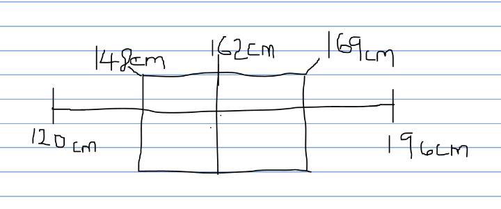
The range of a study is the difference between the maximum and minimum values of the data collected. In the sample, the minimum height value is 120 cm, and the arm span is 90 cm, while the maximum height value is 196 cm and the arm span is 211 cm.

Range of height=196-120=76cm

Range of arm span=211-90=121cm

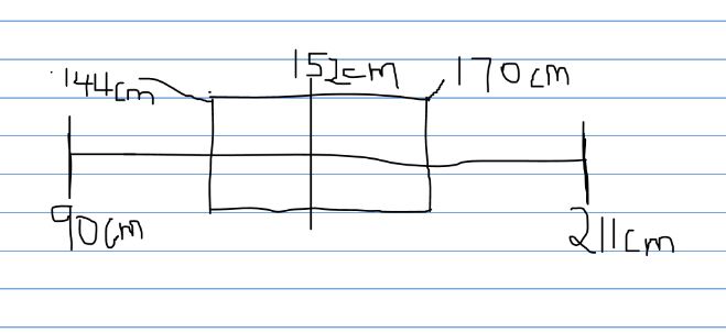
Interquartile Range

The third and first quartile difference is the interquartile range (IQR). To calculate the IQR of the sample, first order the values of height and arm span from the smallest to the greatest (Jones, 2019). Secondly, determine the median, 162 cm for height and 158cm for arm span. Thirdly, the medians of the lower and upper portions are calculated. The median of the lower portion of height is 148 cm, and the arm span is 144, while the upper portion of height is 169.5cm and the arm span is 170. Finally, finding the difference between upper and lower portions to find the IQR is:

IQR of height=169.5-148=21.5cm
IQR of arm span= 170-144=26cm

Linear Regression Model

The regression model describes the relationship between independent and dependent variables by fitting a line to the collected data. Additionally, regression estimates how a change in the independent variable affects the dependent variable (Liu et al., 2019). In the sample data, both arm span and height variables are quantitative. That is why they qualify for regression analysis to determine if there is a linear relationship between them. Simple linear regression is the most appropriate for this study because only one independent variable is analyzed in the sample data.

Since the study’s multiple R is 0.72, it shows a weak positive relationship between arm span and height (see Appendix G). Further on, R² is 0.51; this indicates that 51% of values in the sample fit the regression model analysis (Lukman et al., 2019). Additionally, adjusted R square is not applicable in this study as it is usually used in multiple regression analysis. The standard error of the output is 10.63; since it is a large number, there is less certainty in the regression equation.

The study’s p-value is less than.05, which shows statistical significance. Additionally, it shows that the model is okay, and there is no need to choose another independent variable for the study (see Appendix G). Due to this, we reject the null hypothesis and conclude that there is a positive relationship between arm span and height (Permai & Tanty, 2018). Further on, the coefficients enable the building of the linear equation using y=bx+a. In the sample data, y is the height of the students while x is arm span, and the linear regression formula is as shown below.

Y=Xvariable1*x+ intercept

Substituting a and b with values that are rounded off to four decimal places, the equation will be:

Y=0.5667x+71.5275

Men’s arm spans	Calculation using the equation (y=0.5667x+71.5275)
181 cm	0.5667(181)+71.5275= 174.1002cm
160 cm	0.5667(160)+71.5275= 162.1995cm
165 cm	0.5667(165)+71.5275= 165.033cm
157 cm	0.5667(157)+71.5275= 160.4994cm
177 cm	0.5667(177)+71.5275= 171.8334cm

Using the same method, you can calculate men’s height when provided with their arm span, as shown below.

The above calculations show that men’s arm span can be longer than their heights in some cases, while the height can be longer in others. Additionally, looking at the results, it can be concluded that men’s spans and heights have no significant difference. This indicates a positive relationship between arm span and height regardless of an individual’s gender. Therefore, the calculated examples using linear regression equation support Da Vinci and his Vitruvian Man proportion concept.

Evaluation to Verify Results

The measure of central allows the comparison of height and arm span. In this study, the mean height is 160.07cm, while the arm span is 156.24cm. Additionally, the height median is 162 cm, while the arm span is 152 cm. Further on, the height mode is 165cm, and the arm span is 166cm. The height of students is longer in mean and median than in arm span (Kaliyadan & Kulkarni, 2019). On the other hand, the arm span has the highest mode length than height. Although there is a difference between the measure of central tendency of height and arm span, it can be concluded that they are almost equal because they do not have a significant difference.

Additionally, the measure of tendencies results are accurate, and no method can be used to improve them. The key strength of the mean is considering all height and arm span values to calculate their average. On the other hand, the mean limitation is easily affected by either small or large values. Additionally, the median’s strength is that it cannot be affected by either small or large values (Gupta et al., 2019). The main limitation of the median mainly affecting this study is that the number of students used is even. It can only be calculated by finding the average of two middle numbers. This indicates that the median height and arm span value is not an actual number from the original set. Further on, the mode’s strength is that it can be used in qualitative and quantitative data sets. The mode limitation is that some data sets can have more than one, and others have no mode. Regardless of the measure of central tendency having limitations, they are all applicable in the data sample used in this study.

The main reason for calculating the measure of spread is its relationship with central tendency. In this study, the spread gives us an idea of the mean height and arm span. Since the spread values of range and interquartile range are not large than the mean of height and arm span, the average represents the data (Engledowl & Tarr, 2020). Additionally, the positive differences between fields and interquartile ranges show slight variation in height and arm span, meaning that the two variables are similar.

Since the range and interquartile range of height and arm span are accurate, no method can be used to improve the results. Although the spread is exact, IQR has usually been considered a better measure than range because it is not easily affected by outliers. Since there are outliers in the study, IQR will be used to measure spread (Jones, 2019). Using the IQR shows a positive difference between height and arm spans to indicate a slight variation to imply that the two variables are almost similar. Generally, the measure of the spread explicitly shows the similarity between variables, while central tendency shows an overall description of the sample data.

In the linear regression model, R²is less than 95% which is considered a good fit in the regression analysis model. This can be improved by using the removing outliers method (Kaliyadan & Kulkarni, 2019). Refitting the regression to the remaining points after removing apparent outliers or high-leverage or high-influence data points is a frequent approach in regression. The fit to the remaining points will be enhanced without distorting the data if the removal does not significantly modify the regression function. The outliers in this study are attributable to a nonnormal distribution for the Y sample population or an underlying nonlinear model that fits the overall data better. Using a nonlinear model, which is a linear model with additional X variables, will transform X or Y, fitting the linear model (Liu et al., 2019). This will yield more information than ignoring valid data values. The residual variance for the new fitted linear function may be reduced by deleting a point with a significant residual. However, it will not result in a higher R-square value or a lower P-value for the F test of overall fit.

Using linear regression analysis on the sample data has numerous strengths and limitations. The first strength is that the study performs perfectly for linearly separable data. Secondly, it is easier to implement, interpret, and efficient train. Thirdly, the analysis deals with overfitting perfectly by using regularization, cross-validation, removing outliers, and the reduction method (Lukman et al., 2019). Finally, the regression method extrapolates beyond a particular data sample. On the other hand, the limitation of the analysis is that it has an assumption of linearity between independent and dependent variables. Another limitation is that the analysis is prone to overfitting, noise, and multicollinearity and is sensitive to outliers.

Conclusion

In general, the results obtained from the linear equation show a positive relationship between height and arm span. Additionally, the multiple R shows a positive relation regardless of R^2, indicating that the regression analysis is not fit perfectly. Further on, the p<.05 leads to rejecting the null hypothesis and accepting the alternative hypothesis. All these results acquired from the study tally with the proposed Da Vinci and his Vitruvian mode that an individual’s arm span is equal to his height. Due to this interesting fact, it can be used in clinical practice to facilitate height measurement.

References

Alzyoud, J., Jacoub, K., Omoush, S., & Al-Shudiefat, A. (2021). Da Vinci’s Vitruvian Man, golden ratio and anthropometrics. Italian Journal of Anatomy and Embryology, 125(1), 67-81. Web.

Cadelano, G., Cicolin, F., Enzi, S., Emmi, G., Mezzasalma, G., Busana, M., & Bernardi, A. (2020). Assessing the indoor conditions of a 3rd century AD Roman Domus by dynamic energy simulation and comparison with Vitruvian hypothesis: Preliminary Findings. IOP Conference Series: Materials Science and Engineering, 949(1), 012049. Web.

Engledowl, C., & Tarr, J. (2020). Secondary teachers’ knowledge structures for measures of center, spread & Shape of distribution supporting their statistical reasoning. International Journal of Education in Mathematics, Science and Technology, 8(2), 146. Web.

Gupta, A., Mishra, P., Pandey, C., Singh, U., Sahu, C., & Keshri, A. (2019). Descriptive statistics and normality tests for statistical data. Annals of Cardiac Anaesthesia, 22(1), 67. Web.

Jones, P. (2019). A note on detecting statistical outliers in psychophysical data. Attention, Perception, &Amp; Psychophysics, 81(5), 1189-1196. Web.

Kaliyadan, F., & Kulkarni, V. (2019). Types of variables, descriptive statistics, and sample size. Indian Dermatology Online Journal, 10(1), 82. Web.

Liu, S., Lu, M., Li, H., & Zuo, Y. (2019). Prediction of gene expression patterns with generalized linear regression model. Frontiers in Genetics, 10. Web.

Lukman, A., Ayinde, K., Siok Kun, S., & Adewuyi, E. (2019). A modified new two-parameter estimator in a linear regression model. Modelling and Simulation in Engineering, 2019, 1-10. Web.

Permai, S., & Tanty, H. (2018). Linear regression model using Bayesian approach for energy performance of residential building. Procedia Computer Science, 135, 671-677. Web.