Logistic Regression Results for Data Analysis

Introduction

This paper provides the results of a logistic regression that was run to analyze the data contained in the file “helping3.sav.” The data file is described; the assumptions for the logistic regression are articulated and tested; the research question, hypotheses, and alpha level are stated; and the results of the test are reported and explained.

Data File Description

The data was taken from the file “helping3.sav”. It comprises real research data assessing people’s helpfulness (George & Mallery, 2016). The current paper provides a logistic regression analysis to predict the people’s helpfulness (cathelp, dichotomous: 0=helpful, 1=not helpful, after the modification for analysis by SPSS) as assessed by the friend they tried to help, from those people’s sympathy towards the friend (sympathy, interval/ratio), their anger towards the friend (angert, interval/ratio), the helper’s self-efficacy (effect, interval/ratio), and the helper’s ethnicity (ethnic, categorical; will be dummy-coded in regression; see Appendix). For all the interval/ratio variables, lower numbers represent a lower intensity of the feeling (George & Mallery, 2016). The sample size is N=537. The demographic variables in the data set allow for concluding that the population for the study is rather broad.

Assumptions, Data Screening, and Verification of Assumptions

Assumptions

The logistic regression requires that certain assumptions are satisfied (Field, 2013; Laird Statistics, n.d.):

1. The dependent variable is dichotomous, and comprises mutually exclusive, exhaustive categories; the independent variables are interval/ratio or categorical;
2. There ought to be the independence of observations;
3. There are linear relationships between the continuous independent variables and their logit transformations;
4. There needs to be no multicollinearity in the data.

Verifying Assumptions

Assumption 1

As follows from the “Data File Description” section, the assumption is met.

Assumption 2

The observations are independent–each case represents a different person helping a different friend.

Assumption 3

To test this assumption, it is advised to run a linear regression using the “Enter” method; the regression should include interaction terms between the continuous independent variables and their logit transformations (for instance, their natural logarithms) (Field, 2013, sec. 19.4.1, 19.8.1).

Therefore, three variables were created for this purpose: ln_sympatht, ln_effict, and ln_angert. The results of the analysis are supplied in Table 1 below. It can be seen that the assumption is violated for the variable angert because the interaction is significant (p=.015).

Table 1. Testing the assumption of the linear relationship between the independent variables and their logit transformations.

To address this problem, data transformation procedures can be employed to adjust the independent variables (Warner, 2013). However, this will not be done in the current paper due to the need to follow specific instructions from George and Mallery (2016).

Assumption 4

To test the assumption of non-multicollinearity, it is possible to run a linear regression with the same variables as the main logistic regression while using the SPSS option “multicollinearity diagnostics” (Field, 2013, sec. 19.8.2). It is stated that the tolerance values below 0.1 and VIF (variance inflation factor) values greater than 10 indicate multicollinearity. As one can see from Table 2 below, the analyzed data should have no problems with multicollinearity. Therefore, the assumption is met.

Table 2. Coefficients for collinearity diagnostics.

Screening the Data

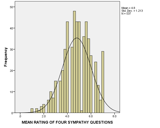
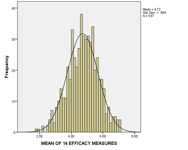
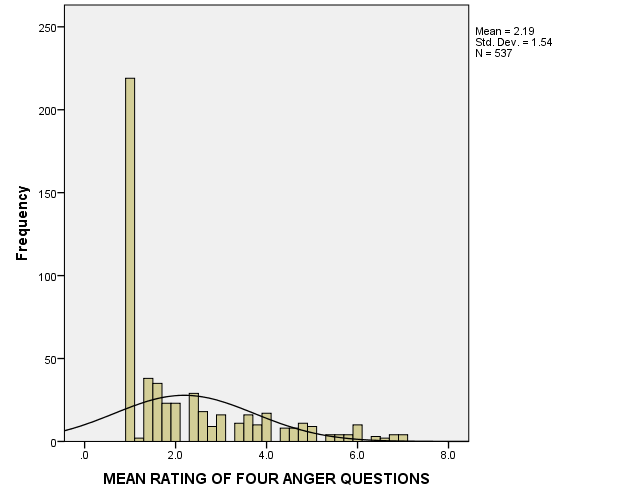
Figures 1-3 below provide histograms for sympathy, effect, and angert variables. It can be seen that sympathy and effect are approximately normally distributed, and there are no apparent considerable outliers. However, the anger variable is not normally distributed due to a large number of values close to 1 (about 220 cases, or nearly 40% of the sample), and because of this, there are some outliers. However, the data will not be transformed, and no outliers will be excluded, for it is needed to follow specific instructions from George and Mallery (2016); also, it is very improbable that such a distribution results from a sampling error.

As for out-of-bounds values, the histograms show that there are no such values in the data.

Inferential Procedure, Hypotheses, Alpha Level

The research question for the given analysis is: “Do any of the following variables: the sympathy, anger, self-efficacy, and ethnicity of helpers–predict the helpfulness as perceived by those they provided help for?” The null hypothesis will be: “None of the following variables: the sympathy, anger, self-efficacy, and ethnicity of helpers–predict the helpfulness as perceived by those they provided help for.” The alternative hypothesis will be: “At least some of the following variables: the sympathy, anger, self-efficacy, and ethnicity of helpers–predict the helpfulness as perceived by those they provided help for.” The alpha level will be standard, α=.05. The hypotheses will be addressed by the χ² of the model and its significance value.

Interpretation

Therefore, logistic regression was conducted using the variables sympathy, effect, anger, and ethnicity as predictors, and the variable can help as the outcome. As was noted, the variable ethnic was recoded by SPSS using the dummy coding technique (see Appendix). The forward stepwise method of entry based on the likelihood ratio was used; the likelihood ratio for variable entry was set at.05, and the likelihood ratio of.10 was used for variable removal.

There were 2 steps in the variable entry. Table 3 below shows how the variables entered improved the model. It can be seen that the first variable added χ²(1)=114.843, p<.001, and the second variable added χ²(1)=29.792, p<.001, resulting in total χ²(2)=144.635, p<.001 of the model.

Table 3. The variables included in the model.

As a result, the variable’s anger and ethnic(1)– ethnic(4) (the dummy variables representing the variable ethnic) were removed from the model (see Table 4 below).

Table 4. The variables which were not included in the model (the final step).

From the Table 5 below, it can be seen that the final model predicted the outcome variable better than the first one, for the -2 Log-likelihood was smaller in the second model (George & Mallery, 2016). It can also be seen that the final model predicted nearly 23.6-31.5% of the variance in the data (Cox & Snell’s R²=.236, Nagelkerke R²=.315). Table 6 below shows that the final model successfully predicted the outcomes in nearly 70.4% of cases.

Table 5. Model summary for the final step.

Table 6. Classification table for the final step.

Only the variables effect and sympathy were retained in the final model, as can be seen from Table 7 below. Effect significantly predicted helpfulness: Exp(B)=3.046, Wald’s test statistic=76.197, df=1, p<.001. Sympathy also significantly predicted helpfulness: Exp(B)=1.596, Wald’s test statistic=27.459, df=1, p<.001. The Constant coefficient for the model was Exp(B)=.001; it had Wald’s test statistic=93.006, df=1, p<.001.

Table 7. Variables in the regression equation at the final step.

Thus, the equation for the regression model at the final step was as follows (George & Mallery, 2016):

ln (Odds (helping)) = ln (P(helping) / P(not helping)) = -7.471 + 0.467×sympatht + 1.114×effict,

or:

Odds (helping) = P(helping) / P(not helping) = e^-7.471 × e^{0.467×sympatht} + e^{1.114×effict}.

Therefore, the null hypothesis was rejected, and evidence was found to support the alternative hypothesis.

A certain limitation related to the fact that the given equations do not take into account the standard error of B, which is displayed in Table 7 above, should be pointed out. Another limitation is related to the entry method (forward stepwise method of entry based on likelihood ratio); purely mathematical considerations were used to select the variables for the final model, which is strongly advised against by Field (2013).

Conclusion

Thus, logistic regression was run to find out whether the sympathy, anger, self-efficacy, and ethnicity of helpers could predict whether they would be assessed as helpful or non-helpful by friends for whom they provided the aid. It was found that sympathy and self-efficacy could predict their helpfulness, whereas the rest of the independent variables could not. Therefore, the null hypothesis was rejected, and evidence was found to support the alternative hypothesis that at least some of the independent variables could predict the helpfulness of helpers.

References

Field, A. (2013). Discovering statistics using IBM SPSS Statistics (4th ed.). Thousand Oaks, CA: SAGE Publications.

George, D., & Mallery, P. (2016). IBM SPSS Statistics 23 step by step: A simple guide and reference (14th ed.). New York, NY: Routledge.

Laerd Statistics. (n.d.). Binomial logistic regression using SPSS Statistics. Web.

Warner, R. M. (2013). Applied statistics: From bivariate through multivariate techniques (2nd ed.). Thousand Oaks, CA: SAGE Publications.

Appendix

Dummy coding of the independent variable ethnic as carried out by SPSS: