Introduction
The polynomial model is an integral concept in mathematics, especially in determining relationships. It is a form of regression where the relationship between dependent and independent variables is determined (Fox & Burks, 2019). For example, the model can identify the relationship between Amazon’s net income/loss and sales. However, there are several steps required to create a polynomial model. One of the steps involves using the data collected to create a scatterplot. To achieve this, a Microsoft excel helps develop a trendline and regression equation. Therefore, creating a polynomial model is a process that starts with developing a scatterplot.
The Steps of Creating a Polynomial Model
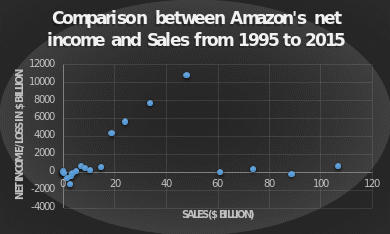
The polynomial model determines the relationship between the independent variable X and the dependent variable Y. There are several steps followed to determine the polynomial model (Fox & Burks, 2019). The first step is using data collected on Amazon’s net income/loss and sales to create a scatterplot, as shown in the figure below. To achieve this, Microsoft excel is used to create a scatterplot automatically. In this case, the dependent variable Y is the company’s net income/loss, whereas the number of sales represents the independent variable X. As a result, the creation of a polynomial model starts with the development of a scatterplot.

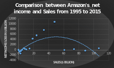
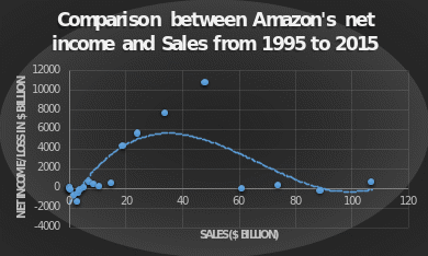
The second step in developing the polynomial model is adding a trendline. A polynomial trendline is a curve that shows how data changes over time. The number of changes in the data can be used to figure out the polynomial order (Fox & Burks, 2019). With the created scatterplot, there is a need to add a trendline. In this trendline, polynomial orders two, three, and four can be used to create the model, as shown in the figures below. To do this, click on one of the points in the scatterplot. After that, right-click, select add a trendline, and a line connecting some points will appear automatically. As a result, excel allows the creation of different trendline based on the order chosen.

Second-order polynomial, also known as quadratic polynomials, is associated with a parabola. In this model, the x variable is squared and has a coefficient and a constant. It is usually used to determine factors in a curve (Fox & Burks, 2019). In addition, it plays an integral role in developing the second-order regression equation. This order distinguishes quadratic equations from the linear regression equation. Furthermore, a second-order polynomial has additional functions that can be used to determine more figures.

A third-order polynomial is different from the second and first order. It is among the high order polynomials due to the existence of X3. This order is of the form of y = ax3 + bx2+ cx + d where ‘a’ is not zero. It is also known as cubic polynomial because it has degree 3. Therefore, polynomial order three is more complex than the first and second order.
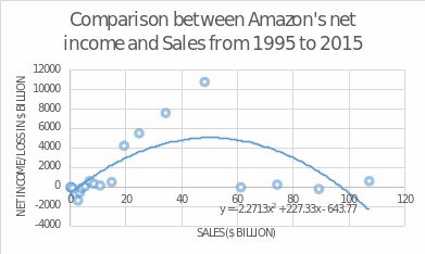
The third step in creating a polynomial model is the creation of polynomial regression equations for each of the orders chosen. On the trendline, it is possible to add various aspects to the scatterplot (Fox & Burks, 2019). One of the features that can be added is the regression equation. For order 2, the polynomial model is shown in the figure below. A second-order polynomial equation was created to predict Amazon’s net income/loss based on sales. The equation for the scatterplot was determined using Microsoft excel’s trendline function. For example, the equation for the model obtained is y = -2.2713x2 + 227.33x – 643.77. In this case, x represents the sales, whereas y is the net income/loss. Therefore, the last step in the process is using the trendline function in excel to generate a polynomial equation.
The order of the polynomial equation was kept as low as possible, and higher-order polynomials were avoided because randomly fitting higher-order polynomials often leads to serious misuse of regression analysis. In most cases, the second-order polynomial is used to determine which input drive responses (Fox & Burks, 2019). As the number of explanatory variables and, by extension, the number of cross-product terms goes up, it is evident that polynomial equations could get much more complicated. In addition, there are limited interactions with more than two factors. This helps keep the equations at a level that is easy to work with (Fox & Burks, 2019). Thus, second-order polynomial was considered in the creation of the model.

Conclusion
The development of a polynomial model begins with creating a scatterplot using data from Amazon’s net income/loss and sales. The polynomial model is an important concept used to determine relationships in figures and aspects. It is a type of regression that looks at the relationship between a dependent variable and an independent variable. For example, the model can determine how Amazon’s sales relate to its net income or loss. However, to make a polynomial model, there is a need to do several things. One of the steps is to make a scatterplot with the collected data. To achieve this, Microsoft Excel is used to make a trendline and regression equation.
Reference
Fox, W. P., & Burks, R. (2019). Applications of operations research and management science for military decision making. Springer, Cham.