Introduction
During the towing of ships on the water, a ship moves between points due to the force exerted on it by another ship; thus, towing means moving one ship at the expense of the forces of another ship. This process may seem easy at first glance, but in reality is associated with a large number of characteristics and aspects leading to increased towing effects or, conversely, problems with movement (Hadler, 2021). During such movement, although the vessel is towed by the application of force, it experiences resistance due to the waves created. At the same time, the water has its own velocity, which can promote or hinder the movement of the towed ship. It follows that this process requires special attention and can be modeled in ship design.
Simulation allows processes and phenomena to be replicated on a miniature scale in order to predict and study the characteristics of the process. Simulating the towing of a real ship means that a mini replica of such a ship is placed on an elongated pool and moved along the line by the force generated by the tensioning devices. This was the experiment in this report, which used the Bulbous Bow (Lony) model, which has a recognizable shape with an elongated leading edge (Prem, 2020), as such a ship. Such a ship was 81 centimeters long and produced a displacement of 1.65 kg when placed on the water. The water speed data of the Bulbous Bow was recorded with sensors and was then used to perform calculations and analysis. Thus, the present work aims to study the mathematical side of the towing process, which includes integration and differentiation operations as well as statistical analysis.
Experimental Procedure
The Bulbous Bow was placed on the water in an oblong pool, and a rope was tied to the front edge of the ship. This rope was stretched and gradually pulled the ship from the starting point to the end point. During this movement, the speed of the water was recorded and recorded in the Minitab and then transferred to Excel (see Appendix). A total of five tests were conducted at different forces and set #5 was chosen as the data for analysis in this work. The values for this test were initially processed, which included removing values where the velocity was zero or fell after reaching a plateau. This was a necessary step to use only useful data and reduce statistical errors. The calculations shown below were performed either manually or with Excel, depending on the context of the problem being solved.
Results and Discussion
Differentiation and Integration
The first part of this paper was to examine the data collected for the fifth test and perform differentiation and integration operations on them. Differentiating a velocity function examines its increment to the change in time, that is, actually taking a derivative that equals acceleration (Dummies, 2021). The faster the ship gained speed, the higher its acceleration will be. During integration, an antiderivative is taken for the original velocity function, which is equal in meaning to the function of the distance traveled. In the case of an indefinite integral, the constant C is added to the expression, but when the limits of integration are set (definite integral), the constant is ignored and the numerical value for the specific distance is found. In other words, the use of the definite integral with the setting of time bounds allows us to answer the question of how many meters the ship has traveled in that time. It is these concepts that were used in the creation of this section of the report. But first, we needed to construct a visual representation of the raw data in the form of a scatter plot: this is shown in Figure 1. Referring to this figure shows that the speed increases almost linearly during the first 6-7 seconds, after which it comes to a plateau and almost does not change.
The same graph reports with high accuracy the regression equation, which describes the behavior of the velocity function. The accuracy is due to the R2 value, which is 0.9959 for this regression model. That is, we can say that the model explains 99.59% of the variance in velocity values. The velocity expression itself has the following form:
![]()
Consequently, the change in velocity occurred in the form of a cubic polynomial, with this polynomial tending to positive infinity at the right end. The function can be differentiated by the time variable to determine the expression for the acceleration:
![]()
As expected, the maximum degree has been lowered as a result of differentiation, so the acceleration is now a quadratic function. With this function the acceleration at any time point can be determined, e.g., at t = 10 sec:
![]()
It follows that by the end of the 10th second, the ship’s acceleration was negative. This is not surprising, since a negative acceleration means that the ship was slowing down, that is, it was slowing down. If we turn to Fig. 1, at this point in time the ship’s speed was practically unchanged but fluctuated within a certain number. Therefore, the negative acceleration is not in doubt.
The original function can also be reintegrated using time bounds. In particular, the value t = 0, that is, the actual start of the test, will be taken as the left boundary. As the right boundary, the maximum value of time fixed for the set is used, that is, t = 13.7725. Then the definite integral will have the following form:
![]()
As previously reported, the definite integral of the velocity function is the distance traveled over the time interval. That is to say:
![]()
There is no longer a constant in this mathematical deduction, so it becomes possible to determine a specific value for the distance traveled by the ship in 13.7725 seconds:
![]()
That is, during this time the ship covered a distance of 11.5621 meters.
Regression
For the moving ship model, resistance values and the maximum speed reached were also measured during each of the five tests: Table 1 summarizes this. At the same time, the table shows the results of calculating the necessary coefficients to calculate the value of the correlation between the variables. Correlation refers to determining the strength and direction of the relationship between two quantitative variables. If this number is positive and as close to 1.00 as possible, it is said that there is a strong positive correlation between the variables.
Table 1: Resistance and velocity measurement data for five tests
To calculate the correlation coefficient, use the standard formula shown below:
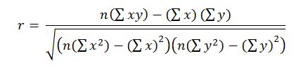
As we can see, these are the values that were calculated earlier and given in Table 1. Thus, all that remains to be done is to substitute the values in the formula:
![]()
That is, looking at the value, we can say that there is a positive, strong correlation between the variables. Squaring this value gives a result of 0.9351, which suggests that the regression model explains 93.51 percent of the variance R/V.
As part of the regression analysis, we need to find the coefficients that define the linear regression function y = mx + b. To do this, use the standard formula for calculating the gradient:
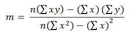
Let us substitute the known values:
![]()
Substituting the point (0.800, 0.220) into the original regression equation gives us a value for the y-intercept coefficient:
![]()
![]()
This means that at zero velocity R/V had a negative value, which did not really make sense. We can create a full regression equation for the five trials, which would have the following form:
![]()
And it can be compared to more reliable Excel calculations, which is shown in Figure 2. They are more dependable because they did not use rounding. We can see that, in general, our calculated coefficients can be called close to what Excel offers.
SNR
In telecommunications, the SNR parameter is used to determine the strength and purity of the transmitted signal. In general, the higher this value is for a particular signal, the less effect noise and interference have on signal quality. In other words, maximum SNRs are recommended for high-precision data transmission. For time-rate data from Part A, we can calculate SNR values. To do this, we need to randomly select fifteen points from the plateau region and use descriptive statistics for them. To be more precise, the following fifteen points were selected as shown in Table 2.
![]()
Table 2. Time (top) and velocity (bottom) data for the fifteen selected points.
The standard formula SNR defines the ratio of the mean value to the standard deviation. Mathematically, this is shown below:
![]()
Therefore, to calculate the SNR, it is sufficient to determine these two values for the velocity function. This was done automatically with Excel. Then the SNR is defined as:
![]()
The calculated value shows that the signal is extremely accurate because the average value is about 120-121 times the standard deviation.
Solution for the Proposed Function
In this part of the assignment, the distance function shown below was proposed for study:
![]()
One of the questions in this section asks how far the ship has traveled by the end of the tenth second. In other words, find the distance for t = 10. This can be done by substituting:
![]()
That is, this ship covered a distance of 1,602 meters in ten seconds. This is significantly more than the ship in part A of this report. The function can also be differentiated to find the expression for the speed:
![]()
This expression can be used to find the speed at a particular point in time, for example after six seconds:
![]()
Or we can find the time at which the speed was zero:
![]()
![]()
![]()
![]()
![]()
![]()
The correct value of time in this case is 1.884 seconds, because time cannot be negative. If we differentiate the velocity function again, we get the expression for acceleration:
![]()
This can also be used to calculate the acceleration at a particular point in time, for example after four seconds:
![]()
Hence, at the end of the 4th second, the acceleration is 42 m/s2. The acceleration is zero when the time is equal to:
![]()
![]()
![]()
![]()
Conclusion
At the end of the report, it should be emphasized that modeling is used to predict processes while conserving resources. In this paper, modeling was used to study the process of towing a Bulbous Bow ship on a water basin. Using function integrations and differentiations, as well as statistical analysis, the following results were found. First, the towing speed is nonlinearly dependent on time. Second, the signal has the highest SNR value. Third, the R/V from V showed a strong positive correlation. Fourth, the detected calculations showed good agreement with the Excel outputs. All of this leads to the conclusion that the findings can be used to further design the Bulbous Bow tow.
Reference List
Dummies (2021) How to analyze position, velocity, and acceleration with differentiation. Web.
Hadler, J. B. (2021) ‘Towing tank’, Access Science, 1(1), pp. 1-9.
Prem (2020) The bulbous bow – why some ships have it and others don’t. Web.
Appendix A
Appendix B